Introduction to Vector Databases

In traditional SQL and NoSQL databases, an index is a data structure that allows for the efficient retrieval of a subset of rows from a dataset. For example, if we have a table of users, we might create an index on the email column to quickly retrieve a user by their email address. Databases can also expose different types of indexes, such as B-tree, hash, and bitmap indexes, each of which is optimized for various data types and access patterns. For example, a B-tree index is well-suited for range queries (i.e. WHERE age > 18), while a hash index is well-suited for equality queries (i.e. WHERE name = 'Alice').

However, traditional databases and indexes are not optimized for storing or querying vector data. Instead, we need a solution where vector data is a first-class citizen. Enter the vector database, a specialized type of database that is optimized for efficiently storing vector data and performing fast similarity searches. A vector database should be able to do three things well:

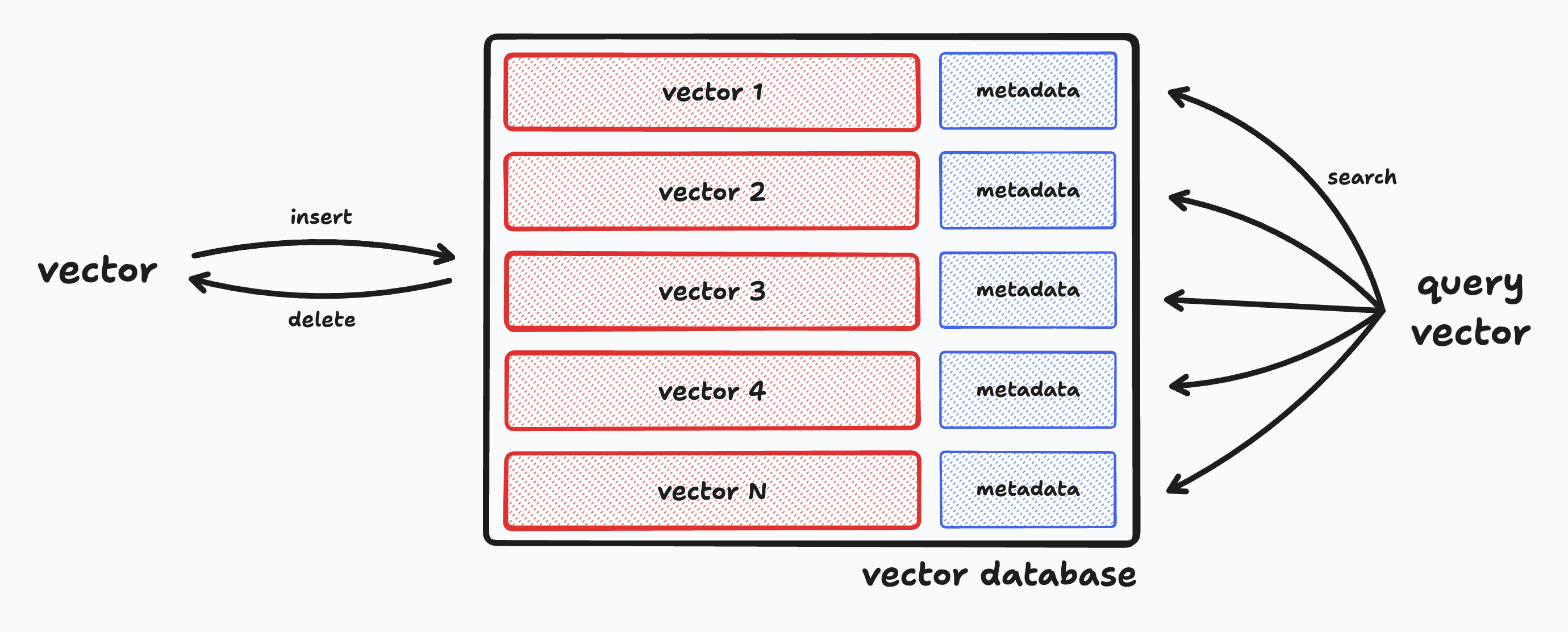
1. Constant time CRUD: A vector database should be able to quickly insert, update, and delete vectors from the database no matter how large the database grows. Semantic search pipelines are often deployed in environments where new documents are added and removed in real time, so the database must be able to keep up with these changes.
2. Fast similarity searches at scale: A vector database should be able to perform similarity searches over millions or even billions of vectors in milliseconds using interchangeable similarity metrics (e.g. cosine similarity, dot product, etc). We'll explore how this is possible using advanced search algorithms and scaling solutions.
3. Metadata storage and filtering: A vector database should be able to store metadata alongside each vector and allow for fast filtering of vectors based on this metadata. For example, we might want to filter vectors based on the date they were inserted into the database or the user who inserted them.

Nearest Neighbor

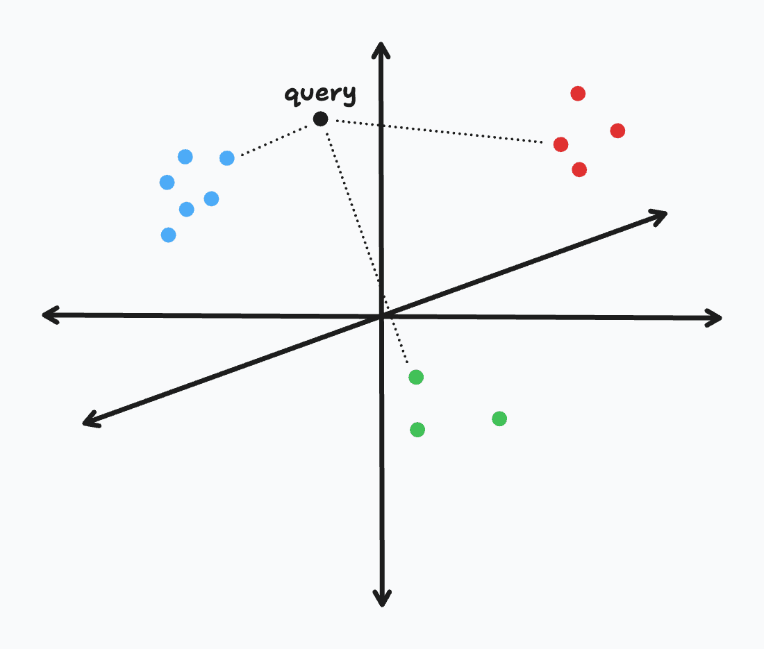
Nearest Neighbor (NN) search is the technical term for the process of finding the closest vector in a dataset to a given query vector. Formally, if we consider vectors as points in a high-dimensional space, NN search is the optimization problem of finding the point in a set that is closest to a given point. This is exactly what we've been doing in the previous lessons when executing our semantic search pipelines. In our case, we've defined "closest" as the embedding vector with the highest cosine similarity to the query embedding vector, but we could also use other similarity metrics such as Euclidean distance or dot product.

A common reframing of nearest neighbor search is to search for to the top k closest vectors instead of the single closest vector; this is known as a k-NN search. In our Paul Graham essay search pipeline, we performed a k-NN search with k=5 to find the top 5 most similar essay paragraphs to our query using cosine similarity. To do so, we used scikit-learn's cosine_similarity function to compare our query embedding vector to each document embedding vector in our corpus.

# exhaustively calculate cosine similarity between query and every document
similarities = cosine_similarity(query_embedding, corpus_embeddings)

# get the indexes of the top k most similar documents
top_k_documents = np.argsort(similarities)[-k:]

By exhaustively comparing our query embedding to each document embedding in the corpus, we are calculating an exact solution. While scikit-learn's cosine_similarity implementation uses highly optimized matrix operations, we are still performing just under 20,000 float point operations for each comparison of two 3,072-dimensional vectors. At the scale of millions or billions of embedding vectors, we'll lose the ability to perform an exhaustive search in real-time (i.e. it will take seconds or minutes instead of milliseconds).

Approximate Nearest Neighbor

To address the performance shortcomings of the brute force approach, we can use an approximate nearest neighbor (ANN) algorithm to take computational shortcuts. ANN algorithms are able to quickly find approximate solutions to nearest neighbor search by trading off some accuracy for a significant speedup. We can quantify the accuracy of an ANN algorithm by calculating the recall of the algorithm:

For example, if we have a corpus of 10,000 documents and we want to find the top 5 most similar documents to a given query, we would have a recall of 0.4 if the algorithm found 2 of the 5 true nearest neighbors.

There are many ANN algorithms that we can use, each of which has its own tradeoffs in terms of accuracy, speed, and memory usage. Typically, every vector database, whether open-source or proprietary, will be built around one of these algorithms. Below, we'll briefly explore some of the most popular categories of ANN algorithms.

Graph-based ANN

Graph-based ANNs, such as hnswlib, construct a graph where each node represents a vector and edges connect close neighboring vectors. One common algorithm is the Navigable Small World (NSW), in which a navigable graph is created by connecting vector nodes in a random manner. To find the nearest vectors, it efficiently traverses the graph from one node to another until the local nearest neighbors are found. Hierarchical Navigable Small World (HNSW) graphs improve upon this by organizing the nodes into layers, with each layer being a selective grouping from the previous one, enabling efficient navigation of high-dimensional data spaces. These methods are known for balancing accuracy and speed in vector searches, though they tend to use more memory than some other techniques.

Clustering-based ANN

Clustering-based ANN methods group similar points together to reduce the search space. Algorithms like k-means and HDBSCAN are used to form clusters, and then search is conducted within these clusters. A popular example is FAISS from Facebook AI Research. The strength of clustering-based methods lies in their ability to handle large datasets efficiently, but they might compromise on accuracy, especially for data points that lie near the boundaries of clusters.

Tree-based ANN

Tree-based ANN methods, such as Spotify's Annoy, hierarchically partition the vector space using tree-based data structures like KD-trees and Random Projection Trees. They are particularly effective in low to medium dimensional data spaces but suffer from the curse of dimensionality, leading to degraded performance in high-dimensional spaces.

Sharding

When handling the largest datasets, even advanced Approximate Nearest Neighbor (ANN) algorithms may struggle in delivering fast similarity searches. To mitigate this, vector databases often employ sharding. This technique, common in distributed systems, horizontally partitions a dataset across multiple machines, or nodes. Sharding plays a critical role in scaling up semantic search pipelines, enabling the distribution of a corpus of embeddings across several machines. This, in turn, facilitates the execution of similarity searches in parallel, significantly enhancing performance and efficiency.

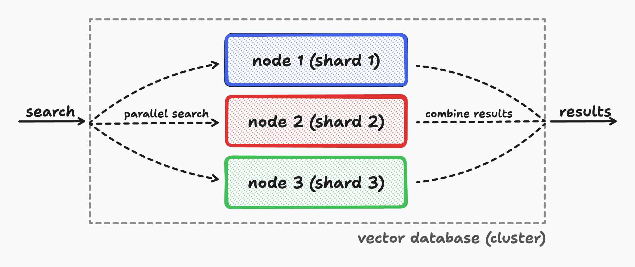
Here are the four key components of sharding in vector databases:

• Data Partitioning: The entire dataset of embeddings is divided into smaller, more manageable segments, each hosted on different nodes. This division can be based on various strategies like range, hash, or even geographic location.
• Parallel Processing: By distributing the data, sharding allows for simultaneous processing across multiple nodes. This parallelism is key to maintaining high-speed search capabilities as the dataset grows.
• Load Management: Sharding helps in balancing the load across the network. Instead of overwhelming a single server with all the data and queries, it spreads these across several nodes, preventing performance bottlenecks.
• Scalability and Flexibility: As the amount of data increases, more shards can be added to the system, offering a scalable solution that grows with the dataset. This flexibility is vital for applications that accumulate data continuously.