Understanding Text Embeddings
Representing Words as Numbers
At the heart of text embeddings lies a surprisingly intuitive concept: representing words as numbers, specifically, multi-dimensional vectors. This numerical representation is not just about assigning arbitrary numbers to words; it's about encapsulating the meaning and context of words into a mathematical form that computers can understand and process. But how do we transition from words, the basic building blocks of language, to numbers that a machine can understand?
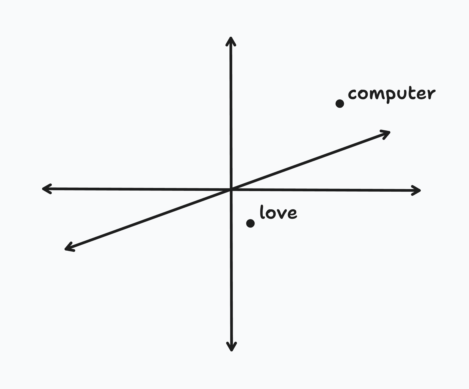
A vector, in this context, is an array of numbers, where each number represents a dimension; a 10-dimensional vector is just an array of 10 numbers. In our word embedding vector, each dimension encodes a different feature or aspect of the word. For example, consider a simple 3-dimensional word embedding model where the first dimension represents a word's association with technology, the second its formality, and the third its emotional connotation.
In such a model, the word "computer" might be represented as the three-dimensional vector , indicating a strong association with technology, a relatively formal usage, and a neutral emotional connotation. On the other hand, a word like "love" might be represented as , showing a weak association with technology, moderate formality, and a strong positive emotional connotation.
A key property of embeddings is that embedding vectors for similar words sit closer together in the embedding space. For example, in our simple 3D embedding space above, we'd expect the embedding vectors for "laptop" and "software" to be geometrically closer to "computer", while words like "hug" and "romance" would be closer to "love".
In practice, we use vectors with far more dimensions, often in the hundreds or thousands. This scale allows for a richer, more nuanced capture of linguistic features, leading to a more precise and meaningful word representation. To construct these high-dimensional vectors, we employ sophisticated algorithms that sift through extensive text datasets, such as the entire English Wikipedia and continuously refine the best numerical representations for words.
Visualizing Text Embeddings
A text embedding, or word embedding in this case, is just a point in a high-dimensional vector space, called an embedding space. To bring this concept to life, let's try to visualize some words in this space.
To do so, we will use a popular pre-trained word embedding model called GloVe. Like other word embedding models, GloVe takes an English word as input and outputs a 50-dimensional embedding vector representing the word. Unfortunately, we can't visualize a point in a 50-dimensional vector space, so we'll use a dimensionality reduction technique called t-SNE to reduce the dimensions of each vector from 50 to 2, allowing us to plot them on a 2D grid. While we won't go into the details of t-SNE here, it's worth noting that this technique preserves as much information as possible and critically maintains the semantic relationships between words.
import numpy as np
import matplotlib.pyplot as plt
import gensim.downloader as api
from sklearn.manifold import TSNE
"""
(1) Let's start by loading a pre-trained GloVe model. We'll download a 50-dimensional version of GloVe that has been trained on 2 billion Tweets and has a vocabulary of 1.2 million words. If you're running this code for the first time, it may take a minute to download since the model is about 200 MB in size.
"""
model = api.load("glove-twitter-50")
"""
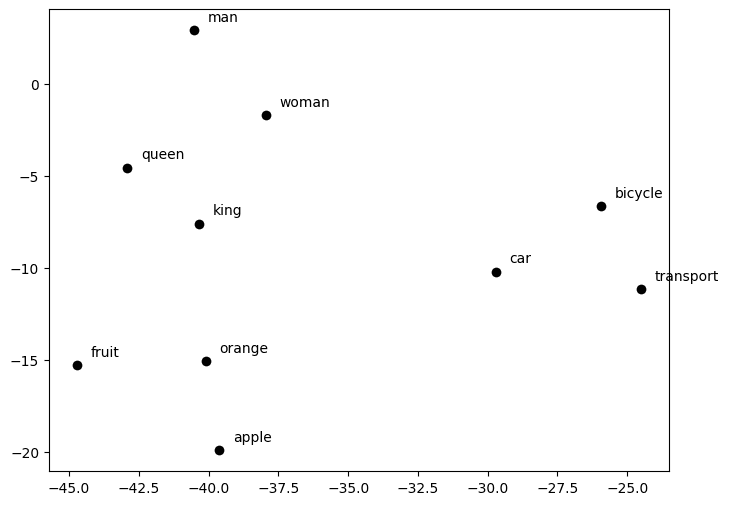
(2) We'll then define some words of interest that we'd like to visualize in our embedding space. We pick words that are related in meaning, such as 'king' and 'queen', or 'car' and 'bicycle', so that we can see how they are positioned relative to each other.
"""
words = [
'king', 'queen', 'man', 'woman', 'apple',
'orange', 'fruit', 'car', 'bicycle', 'transport'
]
"""
(3) Next, let's use the model to "embed" these words, meaning we convert them to our high-dimensional embedding vectors. Each 50-dimensional vector output from the GloVe model is represented as a 50-element NumPy array. By wrapping the output of the list comprehension in a NumPy array constructor, we convert the 10-element list of 50-element NumPy arrays into a (10, 50) NumPy matrix.
"""
word_embeddings = np.array([model[word] for word in words])
"""
(4) Now, since we can't visualize points in a 50-dimensional vector space, we will reduce the dimensions of each vector from 50 to 2 so that we can plot them on a 2D grid. To do so, we will use a dimensionality reduction technique called t-SNE. The scikit-learn library implements an out-of-the-box t-SNE implementation that we can plug directly in here. We set `n_components=2` to indicate that we want the output to be 2-dimensional and call `fit_transform` to generate the new 2-dimensional vectors as a (10, 2) NumPy matrix.
"""
tsne = TSNE(n_components=2, perplexity=5)
word_embeddings_2d = tsne.fit_transform(word_embeddings)
"""
(5) Finally, using Matplotlib, we will plot these new 2-dimensional vectors for each word of interest as points in a Cartesian grid.
"""
plt.figure(figsize=(8, 6))
plt.scatter(word_vectors_2d[:, 0], word_vectors_2d[:, 1], c='black')
for i, word in enumerate(words):
plt.text(word_vectors_2d[i, 0] + 0.5, word_vectors_2d[i, 1] + 0.5, word)
plt.grid(False)
plt.show()
This code will generate the below chart. You'll notice that the points are clustered in four distinct categories: transportation (transport, bicycle, and car), sexes (man and woman), royal names (king and queen), and fruits (fruit, apple, and orange). We can therefore see that the embedding model has successfully captured some sort of semantic relationship between these words.