
More Quantization Formats
Quantization plays a critical role in the open-source LLM community as it effectively opens the door for us to run massive LLMs on commodity GPUs. Consequently, one of the most significant contributions of the community lies in the development and maintenance of pre-quantized models that can be freely downloaded, run locally, fine-tuned, and even shared with others.
As we'll see, these pre-quantized models come in all shapes and sizes — the bitsandbytes quantization format that we learned about above is just the tip of the iceberg. There exist numerous more popular quantization formats that offer diverse accuracy and efficiency trade-offs, specialized support for certain LLM hosting platforms, and even bit widths as low as 1-bit! In this section, we'll take a look at some of the most popular formats and how to use them.
GPTQ
GPTQ is a static quantization format that was introduced in 2022 by Frontar et al. and allows for the highly accurate quantization of LLMs using second-order statistics of the weights. It is designed to be used with a GPU and primarily supports 4-bit and 3-bit block-wise quantization. The format has been integrated into many popular LLM platforms, including the inference engine vLLM, Hugging Face's LLM serving toolkit TGI, and Oobabooga's Text Generation WebUI.
There exist many implementations of the GPTQ algorithm that you might come across, but one of the most popular belongs to a project called AutoGPTQ. AutoGPTQ started off as an independent project but has recently been directly integrated into Hugging Face transformers. Now we can use the same, familiar transformers interface to quantize and load quantized GPTQ-based LLMs. Similar to bitsandbytes, AutoGPTQ functions by replacing the linear layers of a Hugging Face PyTorch model with new GPTQ-quantized layers.
Inference on Pre-Quantized GPTQ Models
As I noted earlier, the most common use case for these quantization libraries isn't to quantize your own models but rather to download pre-quantized models that you can put to work locally. To this effect, the Hugging Face model hub is riddled with models that have already been quantized with AutoGPTQ, just try searching for GPTQ to see for yourself.
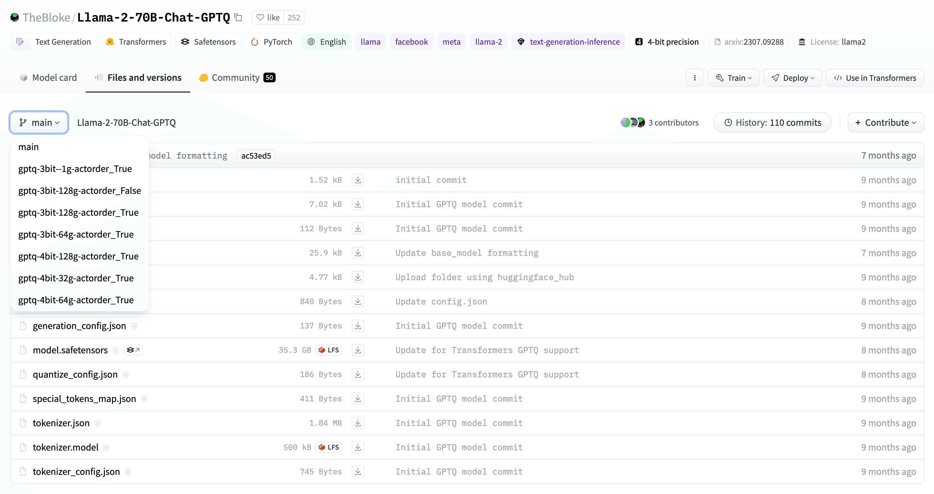
You can find GPTQ-quantized versions of almost any popular open-source LLM, typically with many different bit widths to choose from. For example, TheBloke/Llama-2-7B-Chat-GPTQ is a version of Meta AI's popular Llama 2 7B Chat model that has been quantized with GPTQ. It features a 75% reduction in model size, from 138GB to 35GB, allowing you to run it on a single RTX A6000 GPU!
What's more — if you examine the different revisions (i.e. branches) of that model repository, you'll find both 4-bit and 3-bit quantizations with several different block sizes.
For demo purposes, let's try loading the 7B parameter version of this Llama 2 model. We'll pick the one from the main revision, which has a bit width of 4-bits and a block size of 64. The first (and often the most frustrating step) is to make sure that AutoGPTQ is properly installed. In your Python virtual environment, install the following dependencies:
pip install torch transformers optimum accelerate
We also need to install AutoGPTQ. In theory, you can do this by installing the AutoGPTQ package from PyPI with pip install auto-gptq, but I've unfortunately run into some downstream issues with this method when running CUDA 12. Instead, I recommend installing AutoGPTQ directly from source, which might take a bit longer but guarantees better results:
pip install git+https://github.com/AutoGPTQ/AutoGPTQ.git
The last step is to double check that your CUDA versions are up-to-date. Check the output of nvidia-smi (your CUDA drivers) and python -c "import torch; print(torch.version.cuda)" (the CUDA version PyTorch is using) to make sure that you're using CUDA 12+ across the board. The reason this is important is because GPTQ models, like the bitsandbytes models we saw, are designed to be run on your GPU.
cuda refers to the first available NVIDIA GPU on the system (e.g. model.to("cuda")). If you have multiple GPUs, you can specify the GPU index with model.to("cuda:1") for the second GPU.Now, let's try loading the model from the hub. We'll use the same call to from_pretrained as before but with the model name set to TheBloke/Llama-2-7B-Chat-GPTQ. We'll also pass in a couple extra arguments, including device_map to immediately load the model into GPU memory (instead of needing to do cuda() or to('cuda') later), torch_dtype to set the non-quantized layers to float16 (some extra savings), and revision to target the main branch:
from transformers import AutoTokenizer
from autogptq import AutoGPTQForCausalLM
import torch

model_name = "TheBloke/Llama-2-7B-Chat-GPTQ"

tokenizer = AutoTokenizer.from_pretrained(model_name, use_fast=True)
model = AutoModelForCausalLM.from_pretrained(
	model_name,
	device_map='cuda:0',
	torch_dtype = torch.float16,
	revision="main"
)
Under the hood, the from_pretrained method will download the model files and use the downloaded config.json to detect that the model has already been quantized with GPTQ. It will then load the model using the AutoGPTQ layers and bindings that we installed earlier. The benefit of loading pre-quantized models like this is that (a) we only have to download 4GB of model parameters instead of 14GB (the size of the float32 7B parameter model) and (b) we don't have to worry about the compute-intensive quantization process.
With the pre-quantized model downloaded, we can easily generate text using the same approach as before. The model has already been loaded onto the GPU with device_map so we're good to go:
text = "The meaning of life is"
inputs = tokenizer(text, return_tensors="pt").to("cuda")
outputs = model.generate(**inputs, do_sample=True, temperature=0.5, max_new_tokens=32)
print(tokenizer.decode(outputs[0], skip_special_tokens=True))
The meaning of life is life, is it not? When I was young, I used to think that the meaning of life was all about achieving success, wealth, and fame. But as I grew older, I realized that the meaning of life is to live it, to experience it, to be present in the moment. The present moment is where we find our happiness, our joy, our peace.
Quantizing Models with GPTQ
Oftentimes, you won't be able to find a pre-quantized model on the Hugging Face hub that fits your specific needs. In these cases, you'll want to quantize the model yourself using GPTQ, which is fairly straightforward assuming you have sufficient compute resources.
Since GPTQ is a static quantization algorithm, this process will require a calibration dataset. The calibration dataset should include unlabeled examples that are representative of the inputs that the model will see at inference time. TheBloke, for example, uses part of the WikiText language dataset to achieve a fairly general-purpose quantized model.
Let's now quantize the OPT-350M model from earlier, but this time using static quantization with GPTQ. As mentioned, this process is compute-intensive and can take several hours with larger models and calibration datasets. In our case, with a small model and calibration dataset on a single RTX A6000, this should only take a few minutes:
from transformers import AutoTokenizer, AutoModelForCausalLM, GPTQConfig
from datasets import load_dataset

model_name = "facebook/opt-350m"

"""
We first load the tokenizer for OPT-350M. The `use_fast=True` argument attempts to retrieve a Rust-based tokenizer if available, which is much faster than the default Python-based tokenizer.
"""
tokenizer = AutoTokenizer.from_pretrained(model_name, use_fast=True)

"""
Next, let's build the calibration dataset using the Hugging Face `datasets` library. Here, we load the WikiText dataset and take the first 500 examples from the validation split (with a little additional filtering to remove short examples). In practice, you will need 100-500 examples for calibration, but it's also a good idea to experiment with more if you have the resources to do so.
"""
wikitext_dataset = load_dataset("wikitext", "wikitext-2-raw-v1", split="validation")
calibration_dataset = wikitext_dataset.filter(lambda x: len(x["text"]) > 10)['text']
calibration_dataset = calibration_dataset[:500]

"""
Next, we define our GPTQ quantization config with the `GPTQConfig` class that has been added to `transformers`. We set the bit width to 4 and the group size to 128 (this is the same as block size). The most common group sizes for GPTQ are 128 and 64.

`desc_act` is a more advanced argument that allows GPTQ to quantize rows in the activations matrices in order of decreasing activation, which leads to higher accuracy by placing the quantization error on less important activations. However, when used alongside group size, it can slow down the quantization process significantly. For that reason, we've set it to `False` here.

Lastly, we link the calibration dataset and the tokenizer. The `GPTQConfig` class also includes some built-in calibration datasets from the original GPTQ paper that you can select by passing an identifier string: `wikitext2`, `c4`, `ptb`, etc.
"""
quantization_config = GPTQConfig(
	bits=4,
	group_size=128,
	desc_act=False,
	dataset=calibration_dataset,
	tokenizer=tokenizer
)

"""
Finally, we load the model from the Hugging Face hub using the same routine as before but with the `quantization_config` argument set to our GPTQ config. Under the hood, the `transformers` library will detect that the target model has not yet been quantized (no quantization config in the model's `config.json`) and will perform the GPTQ quantization on the fly using the provided `GPTQConfig`.
"""
model = AutoModelForCausalLM.from_pretrained(
	model_name,
	device_map='cuda:0',
	quantization_config=quantization_config
)
Finally, let's save the quantized model to the Hugging Face hub. This is the exact same procedure as with bitsandbytes models. You have successfully published your second pre-quantized model.
model.push_to_hub(
	repo_id='alexlangshur/opt-350m-int4-gptq',
	revision='main',
	private=True,
	safe_serialization=True
)
That's all there is to it! The Hugging Face community can now take full advantage of your 4-bit GPTQ OPT-350M model. To generate text with the model, simply load it from the hub with from_pretrained and run the same inference code as before.
AWQ
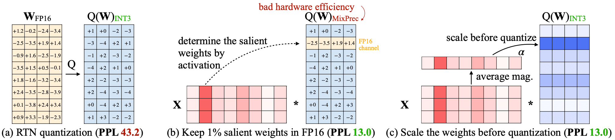
AWQ is a weight-only quantization technique that was introduced in June 2023 by Lin et al.. The key innovation behind AWQ is to leave the most salient weights in float16 (usually the top 1%), which it determines at quantization time by observing the greatest activations over a small calibration dataset. The remaining weights are quantized to int4. Part (b) of the diagram below illustrates this process:
AWQ exclusively supports 4-bit quantization and, like other formats we've seen, is designed specifically for GPU usage. Like GPTQ, it is supported by various inference servers and local text generation UIs, including vLLM and Text Generation WebUI.
Taking inspiration from AutoGPTQ, the most popular implementation of AWQ is a project called AutoAWQ. AutoAWQ has also been integrated into the transformers library so that we can easily load, quantize, and save AWQ models using the same Hugging Face model interface that we know and love.
Inference on Pre-Quantized AWQ Models
Just like GPTQ, you will likely be able to find AWQ-quantized versions of your favorite LLMs on the Hugging Face hub. Take for example the AWQ-quantized version of Llama 2 7B Chat, which is published by TheBloke under the name TheBloke/Llama-2-7B-Chat-AWQ.
To use AutoAWQ, we will follow a similar procedure to what we did with AutoGPTQ. Once you've installed the base dependencies, we need to install two additional packages from source: autoawq and autoawq-kernels. This step might take 5-10 minutes:
pip install git+https://github.com/casper-hansen/AutoAWQ_kernels.git
pip install git+https://github.com/casper-hansen/AutoAWQ.git
Then, let's load a pre-quantized AWQ model from the hub. This time we will choose an uncensored fine-tune of Llama 2 7B called WizardLM 7B. Doing so not only highlights the collaborative capacity of the open-source LLM ecosystem, but also points to one of the key advantages of open-source: centralized LLM providers would never risk serving uncensored models.
from transformers import AutoTokenizer, AutoModelForCausalLM, AwqConfig

model_name = "TheBloke/WizardLM-7B-uncensored-AWQ"

quantization_config = AwqConfig(
	do_fuse=True,
	fuse_max_seq_len=512,
)

tokenizer = AutoTokenizer.from_pretrained(model_name, use_fast=True)
model = AutoModelForCausalLM.from_pretrained(
	model_name,
	device_map='cuda:0',
	torch_dtype=torch.float16,
	quantization_config=quantization_config,
	revision="main"
)
The biggest difference between the inference setup here for AWQ and the one for GPTQ is that we're passing an additional quantization config as we load the pre-quantized model. Earlier, we established that from_pretrained will retrieve the model's config.json from the remote repo to determine if the model has already been quantized (and how it was quantized). This holds true for AWQ models as well, but by passing in an additional quantization config, we can specify additional load-time quantization parameters.
We do this here to take advantage of an AWQ feature called fused modules. Fused modules is an optimization that combines multiple adjacent AWQ-quantized layers into a single module, thus making the forward pass computations more efficient. Normally, GPTQ inference will be faster than AWQ inference since static quantization is typically more efficient than weight-only quantization. However, by fusing the layers, AWQ can achieve similar, if not better, inference speeds! To enable this feature, we set do_fuse to True and fuse_max_seq_len to 512, which is the maximum sequence length that we expect to generate with our fused model.
Under the hood, the from_pretrained method will combine the quantization configs and fuse the pre-quantized model layers as specified. Then, generating text with the model is as simple as before: we tokenize the input, use the model.generate method to autoregressively generate new tokens, and decode the output tokens back into human-readable text:
text = "The meaning of life is"
inputs = tokenizer(text, return_tensors="pt").to("cuda")
outputs = model.generate(**inputs, do_sample=True, temperature=0.5, max_new_tokens=32)
print(tokenizer.decode(outputs[0], skip_special_tokens=True))
The meaning of life is an existential question concerning the significance of existence or consciousness. It has been the subject of philosophy, theology, and humanities. Philosophers such as Jean-Paul Sartre has said, “Existence precedes essence,” which means that the existence of the individual precedes and is more primary than any definitions of identity, purpose, or meaning. Others, like the pre-Socratic philosopher Parmenides, have taken a more cosmological approach to the question, equating existence with being, and concluding that the ways in which we perceive the world cannot capture its true nature.
Quantizing Models with AWQ
Quantizing models with AWQ is a bit trickier since the AutoAWQ integration with transformers currently only supports loading pre-quantized AWQ models. To perform the quantization process itself, we can instead use the standalone AutoAWQ library which conveniently follows a similar interface to transformers.
In exploring GPTQ, we quantized a fairly small model with only 350M parameters. Let's try to increase the challenge a bit by quantizing a much larger and more capable model: Microsoft's WizardLM 2 7B. This model, which is a fine-tune of Mistral 7B Instruct, features 7B parameters and is capable of generating highly coherent and contextually relevant text.
The first thing to note is that AWQ also requires a calibration dataset. However, unlike GPTQ which uses its calibration dataset to derive static quantization parameters for the activations, AWQ uses its calibration dataset to determine which weights to leave in float16. Conveniently, AutoAWQ will automatically perform this step using the pileval dataset if you don't provide your own. Let's take a look at the quantization process:
from transformers import AutoTokenizer
from auto_awq import AutoAWQForCausalLM

model_name = "microsoft/WizardLM-2-7B"

"""
The AutoAWQ interface is a bit different than that of `transformers`, and not all the naming conventions line up perfectly. Instead of directly loading and quantizing the model, we start by simply loading the model with `AutoAWQForCausalLM.from_pretrained`. We then pass in `low_cpu_mem_usage=True` and `use_cache=False` to reduce the memory footprint of the model during the quantization process.

Note that was also include `safetensors=True` because, unlike AutoModelForCausalLM, AutoAWQ does not automatically detect the use of `safetensors` serialization.
"""
tokenizer = AutoTokenizer.from_pretrained(model_name, use_fast=True)
model = AutoAWQForCausalLM.from_pretrained(
	model_name,
	safetensors=True,
	low_cpu_mem_usage=True,
	use_cache=False
)

"""
With AutoAWQ, we can then define our quantization config as the following Python dictionary. The two settings that we have already used are `q_group_size` and `w_bit`, which respectively set the block size to 128 and the bit width to 4.

During our initial foray into mapping functions, we briefly touched on the concept of the affine and symmetric quantization schemes. By setting `zero_point=True`, we are using the affine quantization scheme (i.e. including the zero point in the mapping function), which explicitly centers our range of quantized values around zero. This approach uses slightly more memory but is more accurate.

The `version` argument refers to the version of the AWQ algorithm that we are using. Two versions are supported: GEMM and GEMV. GEMV is 20% faster but only works for batch size 1 and small context sizes. GEMM is more versatile. We'll use GEMM here.
"""
quantization_config = {
	"zero_point": True,
	"q_group_size": 128,
	"w_bit": 4,
	"version": "GEMM"
}

"""
Finally, we quantize the model with the `quantize` method, passing both the tokenizer and our quantization config. During this step, we can optionally pass a `calib_data` argument with either a string pointing to a dataset hosted on Hugging Face or a list of predefined examples. If we don't, AutoAWQ will automatically use the general-purpose "pileval" dataset from Hugging Face. On a single RTX A6000, this process will take around 20-30 minutes.
"""
model.quantize(tokenizer, quantization_config)
Downloading data: 100%|██████████| 471M/471M [00:01<00:00, 295MB/s]
Generating validation split: 0 examples [00:00, ? examples/s]
AWQ: 100%|██████████| 32/32 [17:26<00:00, 32.70s/it]
There it is! Your first AWQ model is now quantized and ready to be used. Since AutoAWQ doesn't implement any of the useful transformers methods for saving models to the hub, we'll need a workaround. Let's save the quantized AutoAWQ model to disk and then load it with transformers so that we can upload it to the Hugging Face hub:
from transformers import AutoTokenizer, AutoModelForCausalLM, AwqConfig

"""
First, let's save our quantized model to disk using AutoAWQ's `save_quantized` method, choosing a name that reflects the origin model and the quantization format. We also explicitly set `safetensors=True` to ensure that the model is serialized safely.
"""
model.save_quantized("WizardLM-2-7B-AWQ", safetensors=True)

"""
Now, let's load the pre-quantized model from disk using `transformers` as we did before. Instead of passing a repo name and revision, we provide the local path to the model files.

At this stage, your system might try to fit both the AutoAWQ and `transformers` models into GPU memory, which could lead to an out-of-memory error. If you're using a Jupyter notebook, I recommend restarting the kernel of the quantization notebook and then running this part separately.
"""
model = AutoModelForCausalLM.from_pretrained(
	"WizardLM-2-7B-AWQ",
	device_map='cuda:0',
	torch_dtype=torch.float16,
	quantization_config=AwqConfig(
		fuse_max_seq_len=512,
		do_fuse=True,
	)
)

"""
Let's wrap things up by uploading the model to a new repository in the Hugging Face hub, along with its tokenizer for the sake of completeness.
"""
quantized_model.push_to_hub(
	repo_id='alexlangshur/WizardLM-2-7B-AWQ',
	revision='main',
	private=False,
	safe_serialization=True
)

tokenizer.push_to_hub(
	repo_id='alexlangshur/WizardLM-2-7B-AWQ',
	revision='main',
)
Go check out the end result of our AWQ quantization process in the alexlangshur/WizardLM-2-7B-AWQ model repository on the Hugging Face hub!
GGUF
GGUF is a highly popular model format that was introduced in August 2023 by @ggerganov alongside the project llama.cpp. The goal of this project is to build a fast and efficient LLM inference engine that can be run locally on top of virtually any compute resource, including commodity GPUs (e.g. RTX 4090), Apple silicon, and even your CPU.
Under the hood, GGUF models have a single core dependency: a machine learning library called GGML that is written entirely in C. GGML effectively acts as the interface between high-level C++ code and low-level CUDA, CPU, and Apple silicon kernels, allowing you to seamlessly run common machine learning operations (e.g. matrix multiplications) on your local device. The llama.cpp project then sits one abstraction layer above this and provides pre-built, GGML-based implementations of common LLM components, such as self-attention.
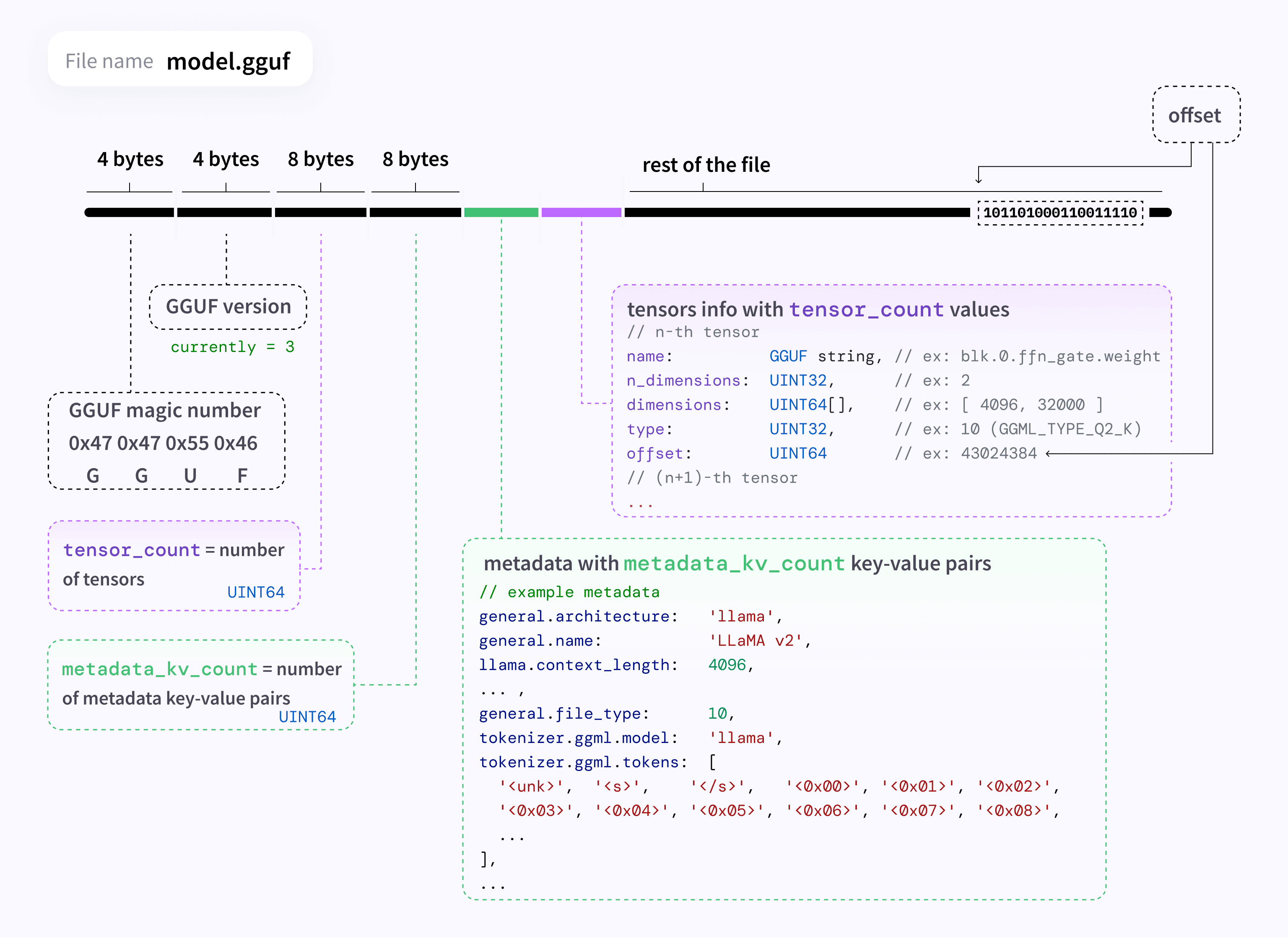
This ties directly into one of the key benefits of GGUF models: they incorporate all the necessary information for running the model in a single portable file. This includes the architecture (i.e. which llama.cpp components to use), weight tensors, prompt templates, tokenizers, and, as we'll see, the quantization method. This is a departure from the PyTorch models that we learned about previously that store the architecture separately from the parameters and spread out the configs and tokenizer across many individual files. Here is a helpful diagram that illustrates how GGUF files are structured:
As mentioned, by using GGML as the backend, GGUF models can be executed directly on your CPU. If you have a GPU available, llama.cpp can offload a portion of the model that fits within GPU memory and run the remaining parts on the CPU. This flexibility is what makes GGUF models so widely adopted and favored.
Quantization Support
Following in the theme of accessibility, one of the most important features of GGUF is its native support for quantization. Over its course of development, GGUF has received support for several quantization methods, each improving on the previous.
Q4_0, Q3_K_S, and IQ2_XXS. These names refer to the quantization type that a GGUF model uses. The two unquantized formats are F32 and F16 for float32 and float16, respectively. Let's take a look at the quantized formats.The first release, known now as the legacy quants, introduced basic, weight-only quantizations that came in three bit widths: 8-bit, 5-bit, and 4-bit. These quantizations are done block-wise in blocks of 32 weights and offer the option of using either the symmetric or affine quantization schemes (i.e. to include or exclude the additional zero point value in the mapping function). The so-called "type-0" quants are symmetric, while the "type-1" quants are affine.
Each GGUF quantization type receives a unique name, which is typically used to describe the GGUF model that we're working with. For example, llama-2-7b-chat.Q4_K_M.gguf is a version of Llama 2 7B Chat that has been converted to GGUF and uses the Q4_K_M quantization type. All quantization types are prefixed with a Q followed by the main bit width. In the case of legacy quants, the suffix is then _0 for "type-0" and _1 for "type-1". Here are some examples:
Q4_0 -> 4-bit, type-0 legacy quant
Q4_1 -> 4-bit, type-1 legacy quant
Q5_0 -> 5-bit, type-0 legacy quant
...
The second release, known as the k-quants, massively improves the quantization accuracy of GGUF models and renders the legacy quants obsolete. It does so by quantizing different parts of the model with different bit widths, keeping the most important parts of the model (usually components of the self-attention layers) in higher bit widths (and "type-1"). A further upgrade of the k-quants method added a device called the importance matrix (or imatrix) which uses a calibration dataset to better determine the most important weights in the model and quantize them appropriately. The imatrix is essential for quantizing to the smallest bit widths.
All k-quant quantization names are prefixed with Q5_K, denoting the main bit width and that the quantization method is k-quant. The suffix (e.g. Q5_K_M) is then one of the S, M, or L sizes, which gives you flexibility in choosing how the more sensitive parts of the model should be quantized. For example, Q3_K_S uses 3-bit quantization for the entire model while Q3_K_M and Q3_K_L use 4-bit and 5-bit quantization, respectively, for the more important model components. Basically, the bigger the size (L > M > S), the more detail is used to encode important layers, producing a larger but more accurate quantized model.
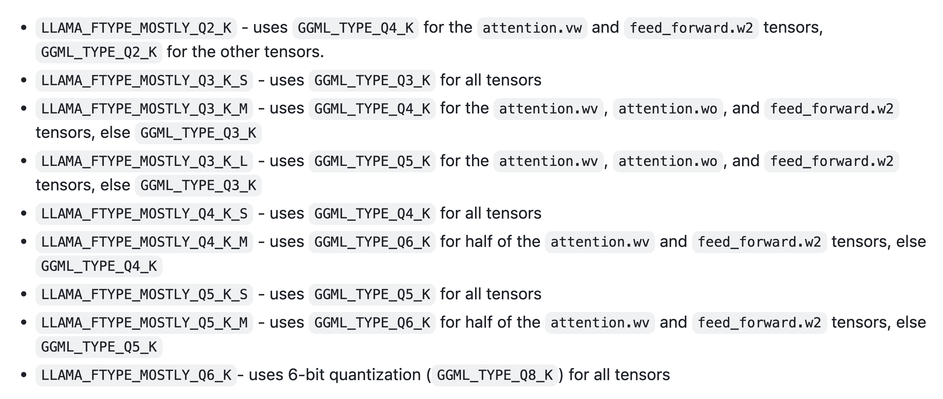
Q3_K_M will use 3.91 bpw, compared to 3.50 bpw for Q3_K_S and 4.27 bpw for Q3_K_L. As expected, none of these bpw values exactly match the base bit width of 3 bits since some of the layers are quantized with 4 or 5 bits.Here is documentation from the llama.cpp repo that shows how the various k-quants, ranging from 2-bit to 6-bit, are structured:
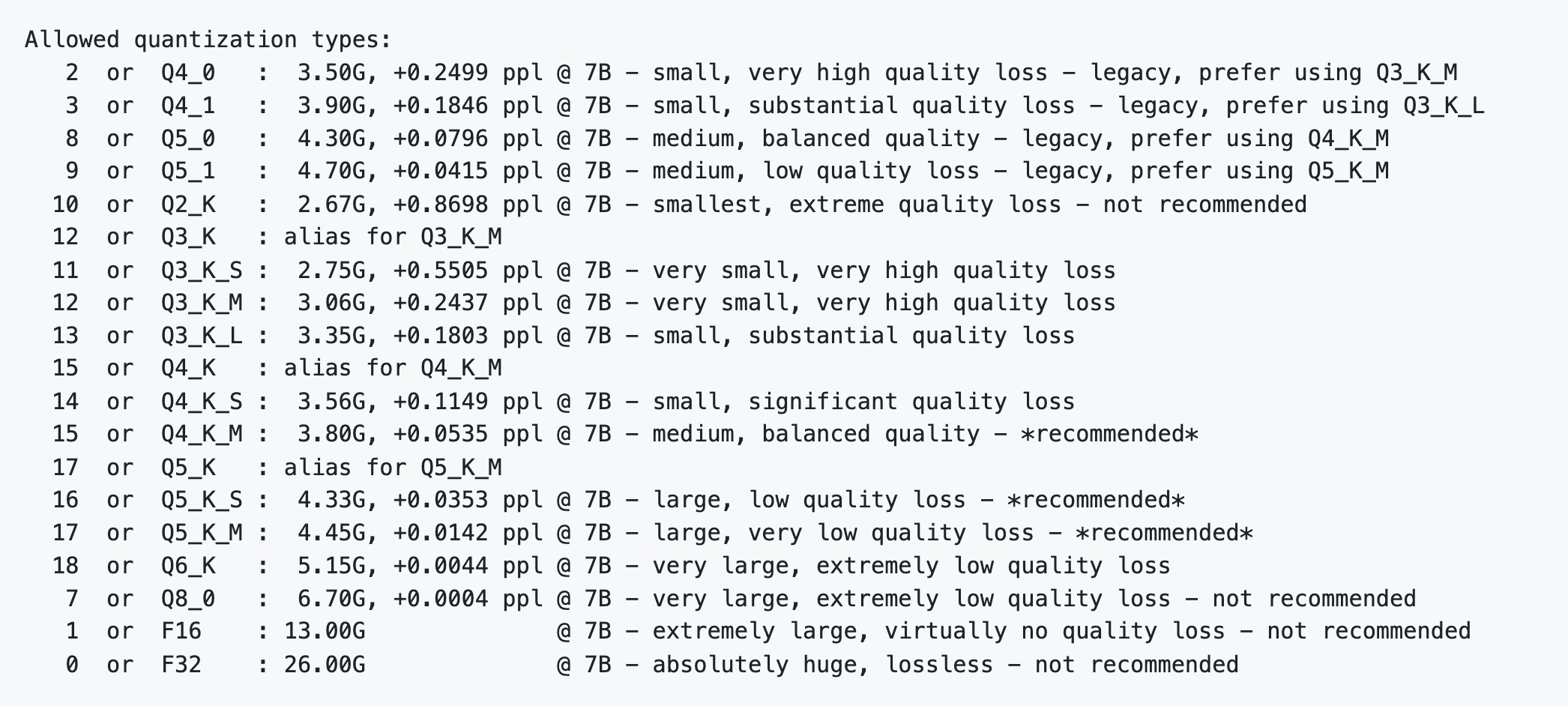
And here is a helpful rubric for understanding which k-quants are recommended. Note that 3.35G refers here to the resulting size of Llama 7B when using that specific quantization type and +0.1803 ppl refers to the marginal perplexity over that of the unquantized model. Perplexity is a common metric that shows how confident a model is in its predictions. An excessive increase in perplexity from the unquantized model typically means that the model is losing accuracy, which might be a sign of over-quantization:
The most recent release that came in January 2024 introduces the I-quants. These quantizations use experimental techniques inspired by the QuIP# paper from Tseng et al. The goal of the I-quants is to achieve sufficient accuracy in the "most extreme compression regimes", namely 3-bit, 2-bit, and even 1-bit. For this reason, llama.cpp requires that you use an importance matrix when quantizing with I-quants.
All I-Quants are prefixed with an I and then follow the same suffix convention as the k-quants. For example, IQ2_S is a 2-bit I-quant that uses 2.5 bits per weight on average. The release also features two new sizes for sub-4-bit quants: XS and XXS. The purpose of these new sizes is to get even closer to the quantization's base bit width without completely sacrificing accuracy. Here is a table that shows the bit widths and bpw for the I-quants:
Inference on Pre-Quantized GGUF Models
Inference on GGUF models looks a bit different than bitsandbytes, GPTQ, and AWQ. Instead of using Python with PyTorch and the transformers library, we need to run GGUF model files alongside the compiled llama.cpp binary. As we'll see later, there are many projects and UIs that are built upon llama.cpp to simplify this process.
The first thing we'll do is download the pre-quantized GGUF model that we want to use. Our model of choice will be Microsoft AI's Phi-3, a cutting-edge 3.8B parameter model that was released in mid-April 2024. If you search "Phi-3 GGUF" on Hugging Face, you'll find many Phi-3 GGUF model repos with different quantization types and sizes, all provided by the community. In our case, we'll double-click on Pruna AI's PrunaAI/Phi-3-mini-128k-instruct-GGUF-Imatrix-smashed repo since it contains over 30 different quantizations to choose from:
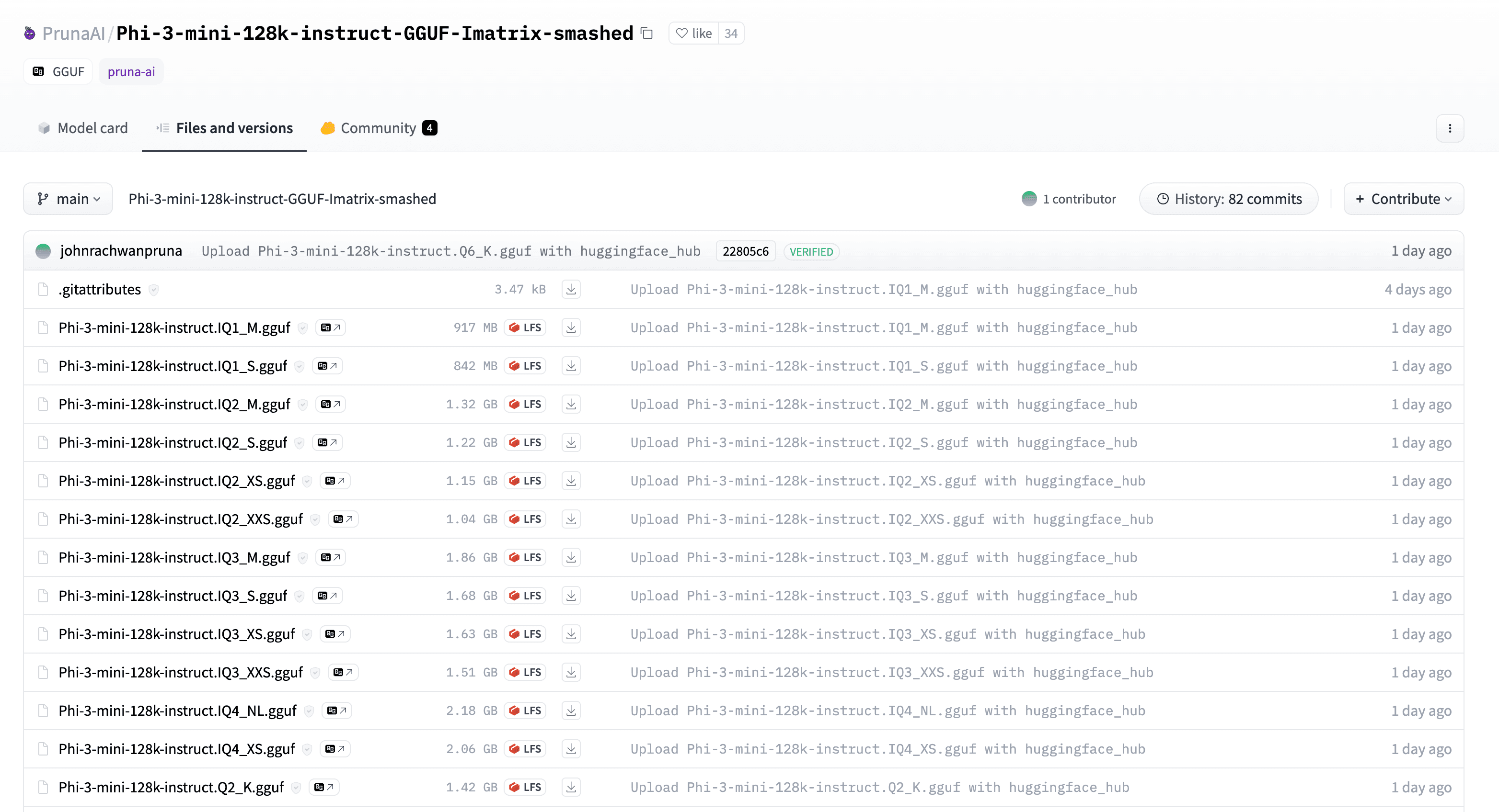
Let's go for a fairly middle-of-the-road k-quant: Q4_K_M. Since GGUF consolidates all model-specific information into a single file, all we need to do is download the correct GGUF file from the repo: Phi-3-mini-128k-instruct.Q4_K_M.gguf.
README.md), you'll notice that Pruna AI explains the methodologies for all their quantizations. Specifically, most of the k-quants and I-quants are quantized with an importance matrix using the WikiText dataset as the calibration dataset. The repo also includes the raw importance matrix that you can use to generate your own GGUF k-quants and I-quants.To download the file, we can either use the huggingface_hub Python library or the Hugging Face CLI. Since we used the Python library earlier, let's try using the CLI to change things up. Start by downloading the CLI with pip install -U huggingface_hub[cli] and logging in with a token from the Hugging Face settings:
huggingface-cli login
Then, we can use the download command to download the model file to a local directory. We specify the repo name, then the specific GGUF file name within the repo, and finally the local directory where we want to save the file (the line breaks are there to make the command easier to read). In this case, the model will end up in ../models/Phi-3-mini-128k-instruct-Q4.gguf:
huggingface-cli download \
	PrunaAI/Phi-3-mini-128k-instruct-GGUF-Imatrix-smashed \
	Phi-3-mini-128k-instruct.Q4_K_M.gguf \
	--local-dir ../models/Phi-3-mini-128k-instruct.Q4_K_M.gguf \
	--local-dir-use-symlinks False
With our file saved locally, let's now run the model with llama.cpp. As I mentioned, llama.cpp compiles to a standalone executable binary that can be run directly on our GGUF files. To get started, download the latest release of llama.cpp from GitHub:
git clone https://github.com/ggerganov/llama.cpp.git
To compile the llama.cpp code into the executable file, let's use make, a build automation tool for compiling code. You can install it with brew install make on macOS or sudo apt-get install make on Ubuntu. Then, navigate to the llama.cpp directory and simply run make:
cd llama.cpp
make
This process may take a few minutes to complete as it crawls through the llama.cpp codebase and generates our executable files. Once done, you will see a new executable file called main! To perform inference on our model, we simply need to invoke it with the path to the GGUF file that we downloaded earlier!
./main \
	--model ../models/Phi-3-mini-128k-instruct.Q4_K_M.gguf \
	--prompt "<|user|>\nWhat is your name? <|end|>\n<|assistant|>" \
	--ctx-size 4096 \
	--n-predict 512 \
	--temp 0.5
<s><|user|>\nWhat is your name? <|end|>\n<|assistant|> I am Phi, an AI digital assistant created by Microsoft.<|end|> [end of text]
There are a few things to take note of here. First, the --prompt flag is used to pass in our input prompt to the model, which you may notice uses an unconventional format. This format is called a prompt template, and it uses special tokens (e.g. <|user|>, <|end|>, <|assistant|>) that the model has used throughout training (specifically, during the fine-tuning phase) to structure its outputs. Prompt templates are particularly helpful in conversational settings by granting the model the ability to delineate exactly what the user has already said and what it has responded with. Additionally, the special <|end|> token allows the model to self-terminate its outputs instead of generating indefinitely.
transformers library, you can then use the handy tokenizer.apply_chat_template method to convert your structured chat into an input that follows the model's prompt template. So, if you wanted to use this approach with Phi-3, you could download the original release at microsoft/Phi-3-mini-128k-instruct, load the model's tokenizer with AutoTokenizer.from_pretrained, and then apply the apply_chat_template function. Check out this guide by Hugging Face for more info. We'll dive into prompt templates in the next lesson when we fine-tune our own models.The --n-predict flag simply specifies the maximum number of tokens that the model should generate, assuming the model doesn't generate an <|end|> token before reaching this limit. Related to this is the --ctx-size flag, which allows you to set the context size that the model will use — this is the maximum number of previous tokens that the model can "pay attention to" at a time when generating the next token, and it includes your initial prompt. So if you keep the conversation going in interactive mode,
For this reason, you should make sure that ctx-size >= n-predict, or the model might start generating incoherent text.
The Phi-3 variant we're using supports a whopping 128k tokens of context using a technique called RoPE scaling. With that said, llama.cpp would need to reserve 49GB of memory to use that much context. If you're using CPU and have a ton of CPU memory, this might be viable (and very slow). However, if you're running on a GPU (which we'll learn about next), good luck fitting that much context into GPU VRAM! Let's keep it at 4096 tokens for demo purposes.
Finally, --temp controls the randomness of the generated text (known as the temperature), with lower values producing more deterministic outputs. In this example, we're just scratching the surface of llama.cpp functionality. I highly recommend you try running the ./main --help command to explore the full range of options that llama.cpp offers, including interactive chat modes, sliders for changing the model behavior, and more.
GPU Inference with llama.cpp
In the output above, I only showed the actual tokens that the model generated. If you run the command yourself, you'll notice that there's actually a ton of additional metadata. In particular, at the very bottom, llama.cpp prints out some timing information that shows how long it took to generate the tokens:
llama_print_timings:      sample time =       0.55 ms /    15 runs   (    0.04 ms per token, 27075.81 tokens per second)
llama_print_timings: prompt eval time =     610.56 ms /    14 tokens (   43.61 ms per token,    22.93 tokens per second)
llama_print_timings:        eval time =    1333.15 ms /    14 runs   (   95.22 ms per token,    10.50 tokens per second)
We see here that the model processed our input prompt at a rate of 22.93 tokens per second and generated new tokens at a rate of 10.50 tokens per second. In the grand scheme of LLM generation, this is super slow. And the reason for this is that llama.cpp is running entirely on your CPU. Quite simply, CPUs are not optimized for running machine learning models. So let's learn how to offload some of the work to a GPU!
Unfortunately, targeting a GPU is not as simple as adding another flag when calling the main executable — we need to completely recompile the binary with CUDA support. This step can be pretty finicky so feel free to reach out if you run into any issues.
First, we need to install the CUDA Toolkit on our machine. This toolkit will enable us to compile the llama.cpp and GGML modules that actually speak to our GPU. If you're running on Debian or a Debian-based distro like Ubuntu, you can do so easily with the commands below. Check out this link for installation instructions on other platforms like Windows.
apt-get update --fix-missing
apt install -y nvidia-cuda-toolkit
The next step will depend on what version of CUDA you have installed, which you can check with the nvcc --version command. If you're running CUDA 11.7+, you should be good to go and can use the following commands to recompile llama.cpp with CUDA support:
# remove the old build
make clean

# recompile with CUDA support
make LLAMA_CUDA=1
If not, you might need to jump through a couple extra hoops. First, head to this page to find out what "compute capability" your GPU supports. For example, if you're running a Quadro P5000, the compute capability will be 6.1. Then, set the CUDA_DOCKER_ARCH environment variable to the appropriate value (e.g. sm_61) and recompile llama.cpp:
# remove the old build
make clean

# export this variable to inform the compiler which GPU architecture to target (sm_61 for Quadro P5000 with compute capability 6.1)
export CUDA_DOCKER_ARCH=sm_61

# recompile with CUDA support
make LLAMA_CUDA=1 PATH="/usr/local/cuda/bin/:$PATH"
Assuming everything goes smoothly and the compilation finishes without any errors, you should now have a new main executable that is capable of running on your GPU. Let's run the same command as before but this time with the --n-gpu-layers flag, which specifies the number of model layers that should be offloaded to the GPU. Phi-3 has about 33 layers, so by setting this value to an arbitary large number like 100, we can offload the entire model to the GPU:
./main \
	--model ../models/Phi-3-mini-128k-instruct.Q4_K_M.gguf \
	--prompt "<|user|>\nWhat is your name? <|end|>\n<|assistant|>" \
	--ctx-size 4096 \
	--n-predict 512 \
	--temp 0.5 \
	--n-gpu-layers 100
If you've done everything correctly, you should see a significant speedup in inference time. On the RTX A6000 that I'm using, I'm now able to generate responses at 140 tokens per second, which is a 14x speedup over the CPU! Here are a few additional lines of metadata output from calling main that are interesting to look at:
ggml_cuda_init: found 1 CUDA devices:
  Device 0: NVIDIA RTX A6000, compute capability 8.6, VMM: yes

...

llm_load_tensors: offloading 32 repeating layers to GPU
llm_load_tensors: offloading non-repeating layers to GPU
llm_load_tensors: offloaded 33/33 layers to GPU
Awesome — when llama.cpp initializes GGML in CUDA mode, it is able to locate the GPU that I'm using and then offload all 33 layers of Phi-3 to it. If you pass in a smaller number to --n-gpu-layers, llama.cpp will offload that many layers to the GPU and run the rest on the CPU. This is a great way to balance the load between your CPU and GPU, especially if you can't fit the entire model in GPU memory. There are also a bunch of more advanced options for those that are lucky enough to have multiple GPUs.
llm_load_tensors:        CPU buffer size =    52.84 MiB
llm_load_tensors:      CUDA0 buffer size =  2228.82 MiB

...

llama_kv_cache_init:      CUDA0 KV buffer size =  1536.00 MiB
llama_new_context_with_model: KV self size  = 1536.00 MiB, K (f16):  768.00 MiB, V (f16):  768.00 MiB
Here is another interesting piece of metadata: a record of exactly how much memory llama.cpp will use on both the CPU and GPU to run Phi-3. The top two lines (with llm_load_tensors) show the amount of memory that will be used for the model's weights. As expected, the weights for every layer have been offloaded to the GPU, consuming about 2GB of GPU VRAM.
The bottom two lines (with llama_kv_cache_init) relate to a feature of transformer architectures called the KV cache. While a detailed explanation of the KV cache is beyond the scope of this lesson, it essentially serves as an inference-time cache that stores intermediate outputs of the model's attention layers from previous token generation steps to accelerate future generations. The KV cache size is directly proportional to the --ctx-size flag that we passed in earlier, as it needs to allocate space for each possible token's attention calculations. In this case, the KV cache has reserved up to 1.5GB of GPU VRAM for a maximum context size of 4096 tokens.
And there you have it! While we don't have time to cover it in this lesson, another fantastic feature of llama.cpp is its native support for Apple silicon. When you compile llama.cpp on a Mac with an M1, M2, or M3 chip, it automatically leverages the Apple Metal API (Apple's equivalent to CUDA for its unified memory and GPU architecture) to run the model. This is a huge win for local LLM inference and Mac users.
Build Your Own GGUF Models
With llama.cpp and GGUF adoption growing throughout the LLM community, you might be wondering how to build your own GGUF models. This process typically involves two steps:
- The first step is to convert a Hugging Face model to GGUF. This can be accomplished with llama.cpp's
convert.pyorconvert-hf-to-gguf.pyscripts, which map the model's PyTorch weight tensors and metadata (e.g. configs, tokenizer, etc) to a single GGUF file. Note that llama.cpp only supports certain Hugging Face model architectures, which you can find in the llama.cpp README.md. - Once you've acquired a valid GGUF file, you can quantize it using the
quantizeexecutable. There are many different quantization types to choose from and you also have the option to use an importance matrix to achieve the smallest bit widths. - Optionally, share your model with the community by uploading it back to the Hugging Face hub! This is a great way to give back.
In the last section, we learned how to perform inference on a pre-quantized GGUF version of Microsoft's Phi-3 mini model. Now, let's take a step back and understand how that model version was created in the first place. Let's start by downloading Microsoft's original Phi-3 model release from the Hugging Face hub. This version is a "traditional" Hugging Face model since it can be used with the transformers library via AutoModelForCausalLM.from_pretrained, which outputs a PyTorch implementation of Phi-3 (see Phi3ForCausalLM for the actual code).
huggingface-cli download \
	microsoft/Phi-3-mini-4k-instruct \
	--repo-type model \
	--revision main \
	--local-dir ../models/phi-3-mini-4k-instruct-hf \
	--local-dir-use-symlinks False
We use the Hugging Face CLI once again here, but this time specify an entire directory to download to since Hugging Face models are spread across many files (unlike GGUF). Take a look in models/phi-3-mini-4k-instruct-hf and you will find the model weights in the safetensors format, along with various configs, the tokenizer, and other metadata.
Now we need to convert this model to GGUF. Since Microsoft published Phi-3 using safetensors, we need to use the convert-hf-to-gguf.py script in the llama.cpp repo to convert it. If your model is in the .bin format, you can use the traditional convert.py script. Let's perform the conversion by passing the directory of the Hugging Face model and the path to the output GGUF file:
python convert-hf-to-gguf.py ../models/phi-3-mini-4k-instruct-hf \
	--outfile ../models/phi-3-mini-4k-instruct.f16.gguf \
	--outtype f16
gguf: loading model part 'model-00001-of-00002.safetensors'
token_embd.weight, n_dims = 2, torch.bfloat16 --> float16
blk.0.attn_norm.weight, n_dims = 1, torch.bfloat16 --> float32
blk.0.ffn_down.weight, n_dims = 2, torch.bfloat16 --> float16
blk.0.ffn_up.weight, n_dims = 2, torch.bfloat16 --> float16
...
Notice how the logs show each PyTorch weight tensor being mapped to its GGUF equivalent? This is the conversion process in action. When it completes, you will receive a new GGUF file named phi-3-mini-4k-instruct.f16.gguf, reflecting the source model, the quantization type, and the model format.
One additional interesting argument to note here is --outtype f16, which tells the conversion script to produce a float16 GGUF model. This is one of three options that you can choose from for the output type: f16, f32, and q8_0. In doing this, we're effectively creating an intermediate model before we fully quantize it. f16 is typically a great choice since it retains virtually all the detail of the original model while being twice as memory-efficient. You can also choose q8_0 to further reduce the memory footprint of this staging model, but this will hurt the accuracy of your downstream quantizations.
The last step is to quantize the intermediate model to our final quantization type. Let's go for something a bit more aggressive this time: Q3_K_M. This is a 3-bit k-quant that uses 4-bit quantization for the self-attention weights. Now all we need to do is call the quantize executable with the path to the intermediate model, the path to the output GGUF file, and the quantization type!
./quantize ../models/phi-3-mini-4k-instruct.f16.gguf ../models/phi-3-mini-4k-instruct.q3_k_m.gguf Q3_K_M
[   1/ 195]                    token_embd.weight - [ 3072, 32064,     1,     1], type =    f16, converting to q3_K .. size =   187.88 MiB ->    40.36 MiB
[   2/ 195]               blk.0.attn_norm.weight - [ 3072,     1,     1,     1], type =    f32, size =    0.012 MB
[   3/ 195]                blk.0.ffn_down.weight - [ 8192,  3072,     1,     1], type =    f16, converting to q5_K .. size =    48.00 MiB ->    16.50 MiB
[   4/ 195]                  blk.0.ffn_up.weight - [ 3072, 16384,     1,     1], type =    f16, converting to q3_K .. size =    96.00 MiB ->    20.62 MiB
[   5/ 195]                blk.0.ffn_norm.weight - [ 3072,     1,     1,     1], type =    f32, size =    0.012 MB
[   6/ 195]             blk.0.attn_output.weight - [ 3072,  3072,     1,     1], type =    f16, converting to q4_K .. size =    18.00 MiB ->     5.06 MiB
In the output, you can watch the quantization process iterate sequentially through each layer in the model, converting the weights from float16 to the specified quantization type. Notice how blk.0.ffn_up.weight tensor (from the feed-forward layer) is quantized to 3-bit quantization, while blk.0.attn_output.weight (from the attention layer) is quantized to 4-bit? The output also tells us just how much each tensor is compressed.
You might be wondering about 2-bit and 1-bit quants, especially using the latest I-quants method. Given the sensitivity of these quantizations, llama.cpp requires that you use an importance matrix when quantizing to these bit widths:
Please do not use IQ1_S, IQ1_M, IQ2_S, IQ2_XXS, IQ2_XS or Q2_K_S quantization without an importance matrix
If you have an importance matrix available, such as the one Prune AI uploaded, you can pass it to the quantize executable with the --imatrix flag. If you want to generate your own importance matrix using a custom calibration dataset, you can do so with the imatrix executable (although be aware that this process will take a while).
Let's wrap up by running our quantized model with llama.cpp. We'll use the exact same command as before, offloading all 33 layers to the GPU, and pointing to our freshly minted Phi-3-mini-4k-instruct.q3_k_m.gguf GGUF file:
./main \
	--model ../models/phi-3-mini-4k-instruct.q3_k_m.gguf \
	--prompt "<|user|>\nExplain LLM quantization in 5 words.<|end|>\n<|assistant|>" \
	--ctx-size 4096 \
	--n-predict 512 \
	--temp 0.5 \
	--n-gpu-layers 100
<s><|user|>\nExplain LLM quantization in 5 words.<|end|>\n<|assistant|> Layer-wise compression of weights.<|end|> [end of text]
If you followed along this far, you're now an official llama.cpp expert! I highly recommend you go explore the llama.cpp Github repo to learn more about the project. For example, one capability that we didn't cover but is worth mentioning is llama.cpp's HTTP server mode, which allows you to serve your models over a REST API. Pair this with a platform like Docker and you have a scalable, GPU-accelerated LLM inference service at your fingertips.
Industry Adoption
In the last few years of operating, llama.cpp and GGUF have become a staple in the LLM community. As we've seen, the Hugging Face hub is filled with pre-quantized GGUF models, ranging from official releases by tech giants like Microsoft to experimental fine-tunes by community members.
Beyond the distribution of models, llama.cpp has also become a popular choice of backend for local chat interfaces, likely due to its portability and diverse options for hardware acceleration. Some of the most popular names in the space that leverage llama.cpp under-the-hood include Oobabooga's Text Generation WebUI, Nomic AI's GPT4All, LM Studio, and KoboldCpp.
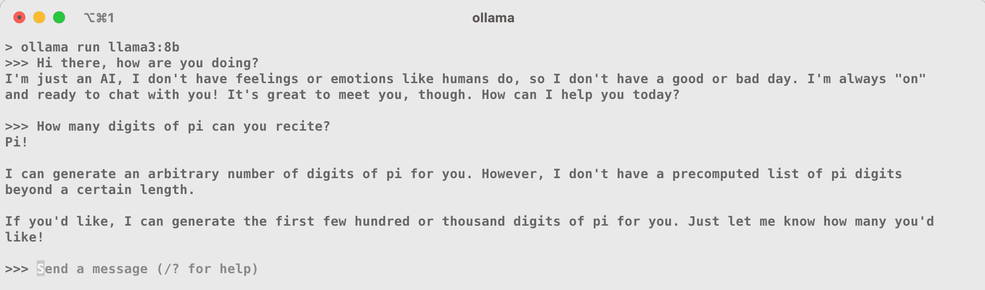
And, of course, a special shoutout to Ollama which allows you to run GGUF models locally via llama.cpp with zero setup. Here I am using Ollama to run Llama 3 8B locally on my M1 Mac that has only 16GB of unified memory:
Annoyed with CLI commands and GUIs? Want to run GGUF models in Python? No problem. Here are a couple additional mentions from the llama.cpp ecosystem:
- llama-cpp-python is a simple project that provides Python bindings for llama.cpp, allowing you to do everything we've done in this lesson but using Python.
- ctransformers is an effort to build a version of the
transformerslibrary that replaces its PyTorch backend with GGML, allowing you to run GGUF models in Python using the familiarAutoModelForCausalLM.from_pretrained.
EXL2
Before wrapping up, there's one more quantization format that I want to mention: EXL2. Just as GGUF is the model format for llama.cpp, EXL2 is the format for a project called exllamav2. The author turboderp calls exllamav2 a "more memory-efficient rewrite of the HF transformers implementation of Llama for use with quantized weights."
As such, exllamav2 is similar to the AutoGPTQ and AutoAWQ libraries in that it uses PyTorch as its backend and stores the model and tokenizer in the same format as Hugging Face transformers. The biggest difference, however, is that exllamav2 implements its own interface for interacting with EXL2 models and hasn't yet been directly integrated into the transformers library. This will likely change in the future.
exllamav2 uses a quantization algorithm that closely resembles GPTQ's static quantization but can mix quantization levels to obtain average bit widths anywhere between 2 and 8 bits. One of the most revered features of EXL2 is its speed. In controlled benchmarks, EXL2 has been shown to be faster than GPTQ, AWQ, and GGUF.
Let's get started by installing exllamav2. Just like the other libraries, we'll install it from source, along with its dependencies, by cloning the repository and installing the requisite packages:
git clone https://github.com/turboderp/exllamav2
cd exllamav2
pip install -r requirements.txt
pip install .
Once installed, let's use the Hugging Face CLI to download a pre-quantized EXL2 model. If you head to the model repo for turboderp/Mistral-7B-instruct-exl2, you'll notice that each revision corresponds to a different average bit width. Let's go for the 2.5 bpw version, which is a whopping 82% reduction in size from the original 15GB Mistral 7B model:
huggingface-cli download \
	turboderp/Mistral-7B-instruct-exl2 \
	--repo-type model \
	--revision 2.5bpw \
	--local-dir ../models/Mistral-7B-Instruct-2.5bpw-EXL2 \
Now, we can use the simple test_inferece.py Python script in the root of the exllamav2 repo to run inference on our model. This script implements a fairly simple CLI interface for running EXL2 models using the main exllamav2 components. If you wanted to build your own Python application for running EXL2 models, you'd recycle the code from this script. Let's run our model with the prompt "Happy birthday!" and generate 64 tokens:
python test_inference.py \
	--model_dir ../models/Mistral-7B-Instruct-2.5bpw-EXL2 \
	--prompt "<|im_start|>user\nHappy birthday!<|im_end|>\n<|im_start|>assistant\n" \
	--tokens 64
 -- Model: ../models/Mistral-7B-Instruct-2.5bpw-EXL2
 -- Options: []
 -- Loading model...
 -- Loaded model in 2.1351 seconds
 -- Loading tokenizer...
 -- Warmup...
 -- Generating...

Happy birthday! We're celebrating with a delicious, spicy, and flavorful tacos and margaritas party!

Tacos:
We'll be serving up traditional tacos, as well as some unique twists on the classic. Here are some of the taco options we'

 -- Response generated in 0.54 seconds, 64 tokens, 118.66 tokens/second (includes prompt eval.)
How about that? exllamav2 will automatically detect and leverage the available GPU, achieving 120 tokens per second on a 7B model! This is about as fast as GGUF was able to generate text on a model of half this size (Phi-3 with 3.8B parameters).
Since EXL2 is a fairly recent format, we won't go into the details of how to build your own EXL2 quantized models. But, if you are interested, all you need to do is use the provided convert.py Python script to convert and quantize a float16 model to EXL2. Simply specify the input and output model directories, your calibration dataset in Parquet format, and the target bit width:
python convert.py \
    -i ../models/hf-model-dir \
    -o ../models/exl2-model-dir \
    -c calibration-dataset.parquet \
    -b 5.0
Comparing Formats
When seeking to quantize an LLM, the first big consideration to think about is the intended use case for the model. This can help you eliminate certain quantization formats right off the bat.
Local Inference
One example of a use case might be local inference. If your goal is to deploy an LLM for local chat purposes, you might want to consider GGUF since llama.cpp forms the backbone of many chat interfaces. Some of the most popular UIs include Ollama, LM Studio, and GPT4All, just to name a few.
A second consideration that ties directly into this one is the hardware you have available. For example, if you're running on a Mac, you should use GGUF since llama.cpp features optimizations for Apple silicon. If you have a GPU available but can't fit the entire model in GPU VRAM, llama.cpp also offers the flexibility of offloading only a subset of the model to the GPU. On top of all this, GGUF is the most popular quantization format and is surrounded by a big developer community.
However, if you can fit the entire model in VRAM, an option like GPTQ or AWQ might be more appropriate since they are typically faster and are also supported by a wide range of chat interfaces. Following in this vein, if your main goal is to achieve the fastest inference times possible, EXL2 might be the best choice since it has been shown to be faster than GPTQ, AWQ, and GGUF in controlled benchmarks. The biggest downside with EXL2 is that exllamav2 is fairly young, so there aren't as many pre-quantized models and you'll likely have to do some technical heavy lifting to get it up and running.
Production Inference
If you're looking to serve an LLM externally to customers, you should look into a production inference engine such as vLLM or Text Generation Interface (TGI). These engines can be spun up as high-performance servers and feature a wide range of production optimizations such as continuous batching and paged attention.
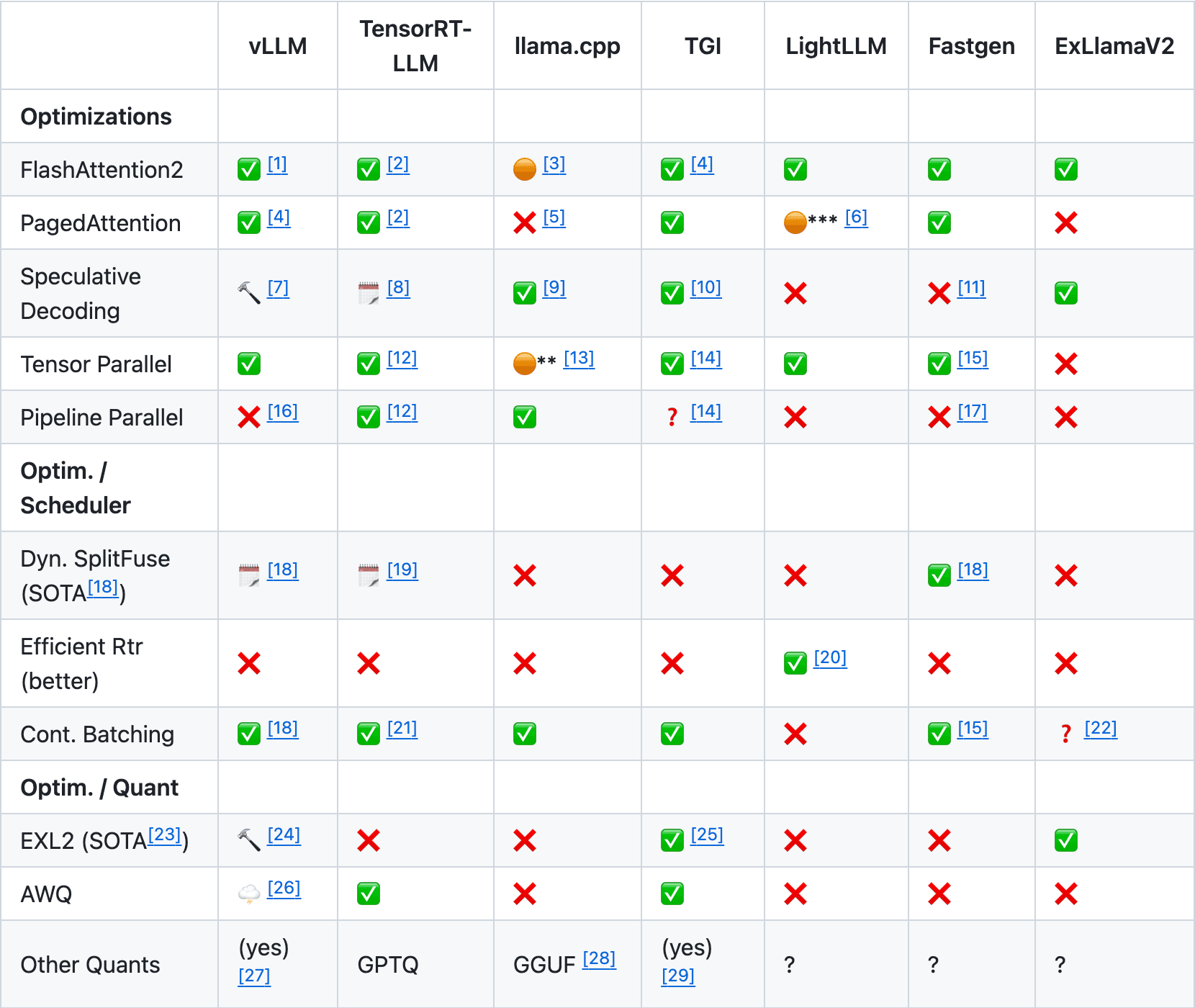
vLLM is often considered the king of inference performance and supports a variety of quantization formats, including GPTQ and AWQ. TGI, on other hand, is an offering from Hugging Face that isn't quite as fast but supports more recent formats like EXL2. Here's a helpful table that summarizes the main inference engines and their relative strengths (the full table is here):
Quantization Level
When planning the level of quantization to apply to your model, the most important factor is the size of the quantized model relative to the available memory on your device(s). A good starting rule of thumb is that a more heavily quantized large model will outperform a less quantized small model. For example, a 4-bit 70B model will be more useful than a float16 13B model, despite being similar in absolute size.
The next thing to think about is the retention of accuracy in the quantized model compared to the unquantized model. The most common method to measure this is perplexity, which we discussed briefly earlier. As a reminder, perplexity is a positive numerical value that measures how confident a model is in its predictions. The higher the perplexity, the more uncertain the model is. To illustrate this, here is a helpful chart that shows how various GGUF k-quants for different model sizes compare in terms of perplexity:
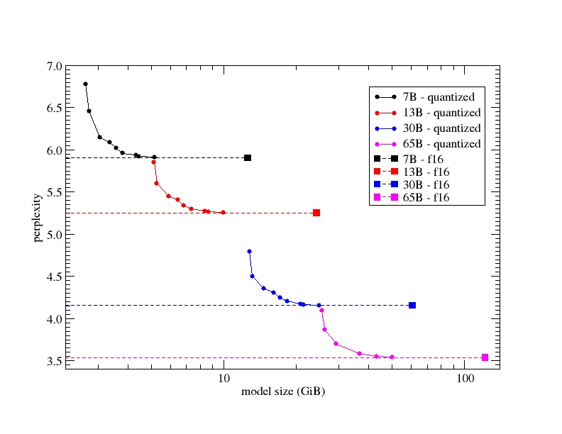
This chart tells us that as we increase the bit width of the quantization, the perplexity of the model will converge to that of the unquantized float32 model. Conversely, as we decrease the bit width too far, the marginal perplexity increases and the model's performance will degrade exponentially. In decreasing the bit width, we reach a point where we may as well use a less quantized version of a smaller model. For this reason, it is typically not recommended to use quantizations below 4 bits (unless they work for your specific use case).
Here is another helpful chart that compares the perplexity and VRAM of a single model quantized with many different 4-bit quantization formats:
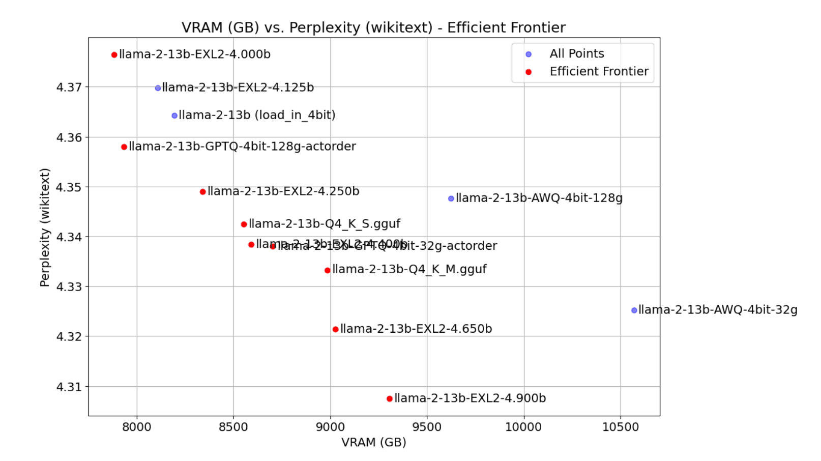
As you can see, the chart establishes an efficient frontier between perplexity and VRAM. AWQ is lower in perplexity but sees higher VRAM usage, while GPTQ is higher in perplexity but is often smaller in memory. However, for the most part, the frontier is dominated by GGUF and EXL2, which offer the best trade-off between perplexity and VRAM.
The above chart is just one section of a larger blog post by Oobabooga that provides the most comprehensive analysis of LLM quantization formats that I've seen. I highly recommend checking out the full blog post to develop a better intuition for the trade-offs between different formats. Beyond this, the best thing you can do is experiment with your own models at different quantization levels and formats to see what works best for you.