Quantization: 0 to 100

The main benefit of LoRA, as we saw previously, is to significantly reduce the number of parameters that need to be updated at each fine-tuning training step. In our example, we saw that LoRA could reduce the number of trainable parameters for Mistral 7B by 99.7%, allowing us to train the model much faster and with commodity GPUs. We've therefore solved the compute problem.

However, the issue of GPU memory remains. Although we reduced the number of trainable parameters, LoRA still requires us to store all of the base model's fixed parameters in GPU memory. Recall the layer output formula that we derived, where $X$ is the layer input and $Y$ is the layer output:

Only the $M$ and $N$ LoRA weight matrices will actually be updated during fine-tuning, but we still need the base model's $W$ weight matrix and $b$ bias matrix in order to compute the layer's outputs. Therefore, all of these matrices must fit in GPU memory.

In the case of a model like Llama 7B, which is on the smaller end of the LLM size spectrum, the base model's parameter alone can occupy over 28GB of memory! The most powerful commodity GPUs (e.g. RTX 4090) have at most 24GB of memory, meaning this would only work on multi-GPU setups or professional-grade GPUs. Enter quantization: an approach to massively reduce the size of LLMs so that they can easily fit in GPU memory.

The Key Insight

In a conventional LLM, every single parameter is represented as a 32-bit floating point number, often referred to as float32 or fp32. This is a very high-precision format for representing real numbers (e.g. 1.2345), but it's also very memory-intensive as it requires 32 bits (4 bytes). This is also sometimes known as "full precision".

The insight behind quantization is that we can represent parameters using a lower-precision format, such as 8-bit integers (int8), without significantly impacting the model's performance. In other words, LLMs don't need all the flexibility that 32-bit floating point numbers provide. By reducing the number of bits used in each parameter, the overall model gets a lot smaller (4x smaller in the case of float32 to int8 quantization) and consumes less GPU memory. On top of this, compute hardware is often optimized for integer arithmetic, allowing quantized models to run faster and with less power consumption.

The Image Compression Analogy

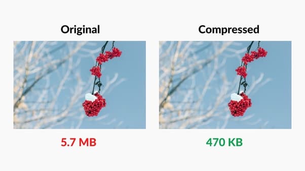
A great way to intuit what quantization is doing is to think about image compression. When we compress an image using a technique like JPEG, we're reducing the amount of information used to represent each pixel, resulting in an overall smaller file size. Despite being a lossy operation (i.e. some information is lost in the process), the compressed image retains roughly the same quality as the original.

Similarly, quantization involves reducing the amount of information used to represent each parameter in the model, resulting in a smaller and more portable model that roughly retains the unquantized model's performance.

Starting with Floating Points

The absolute simplest way to quantize a model is to go from float32 to float16 (fp16 or "half precision"). To understand why this is the case, let's break down how floating point numbers are represented in memory.

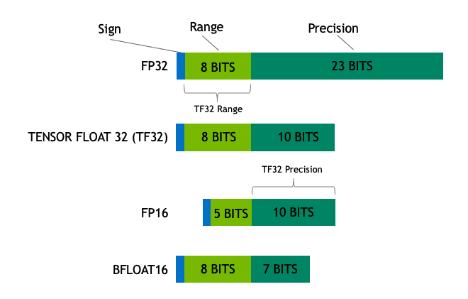
Floating point numbers follow a unique representation scheme that allows them to represent a wide range of values with varying levels of precision. Each 32-bit floating point number is composed of three parts: the sign bit, the exponent, and the mantissa. The sign bit determines whether the number is positive or negative, the exponent determines the scale of the number, and the mantissa determines the precision of the number.

Given these three components, we can calculate the value of the float32 number using the following formula, where $s$ is the sign bit, $e$ is the exponent (combined with a term called the bias), and $m$ is the mantissa (calculated using its bits $m_1$, $m_2$, etc):

Since float16 numbers follow this same representation scheme, it is very simple to convert float32 values to float16. Not only does this mean half the memory consumption, but GPUs also run float16 computations faster. On top of this, most machine learning backends can perform this conversion out of the box. For example, in standard PyTorch, you can quantize a model to float16 in a single line:

model = ... # load your torch model
model.half() # float16 model that uses half the memory

The one caveat is that float16 uses only 5 bits for the exponent (vs 8 bits in float32), which means that float16 numbers have a smaller range of representable values. This can lead to overflow (when the number is too large to be represented) or underflow (when the number is too small to be represented). For example, if you do 1000.0 x 1000.0 in float16, you'll get NaN ("not a number") because the result is too large to be represented. However, this can usually be avoided with techniques like gradient and loss scaling.

Another remedy to this issue is to use a newer format called bfloat16 (bf16), which uses the same 8-bit exponent as float32 but only 7 bits for the mantissa. We therefore sacrifice precision in order to match float32's range of representable values. This format is supported on newer CUDA-based GPUs like the NVIDIA A100, the 30 series GPUs (e.g. RTX 3090), and the 40 series GPUs (e.g. RTX 4090).

Mapping Functions

Experiments have shown that inference on a float16 model produces nearly identical results to inference on a float32 model, but with half the memory consumption and faster compute times. Can we go even smaller than half precision?

The answer is yes — but it no longer makes sense to use floating point numbers. Instead, we can use integers. The problem therefore becomes how to map large floating point values to much smaller integer values and vice versa. This is the essence of quantization.

Let's consider the example of 8-bit quantization, which is the process of converting a float32 model to an int8 model ("quarter precision"). To perform the conversion, we define a mapping function $Q(\cdot)$ that maps every float32 parameter $r$ to a corresponding int8 value $Q(r)$:

Here, $s$ is a float32 value called the scaling factor. And $z$ is an int8 value called the zero point that corresponds to the value 0 in float32 space. Together, we call these two values the quantization parameters. Intuitively, the mapping function first scales the float32 value down to the int8 range and then shifts it so that it is centered around 0 (hence, why we call it the "zero point").

Let's consider an example where we have three float32 parameters in our model: 2, 3.5, and 3.75. We'd like to quantize our model to int8. To do so, we will map the range $[a, b]$ of the model's float32 values (in this case $[2, 3.75]$) to the range $[a_q, b_q]$ of all possible int8 values (i.e. $[-128, 127]$). Here is what the pre-quantized values looks like:

To quantize our float32 values, we first need to calculate our quantization parameters. The scaling factor $s$ is defined as the ratio of the input range to the output range. Once we calculate $s$, we can derive the zero point $z$.

Now, let's perform a quantization step by plugging in a float32 value into our mapping function to get the corresponding int8 value. We will quantize the float32 value 3.5 to int8:

We can repeat this process for all the float32 values in our model to attain the quantized model. Below is what the quantized values look like on the same number line. Notice that we projected the float32 values onto the range of all possible int8 values by mapping $a$ to $a_q$ (i.e. 2 to -128) and $b$ to $b_q$ (i.e. 3.75 to 127).

By rearranging the mapping function, also known as the quantization function, we can derive the dequantization function. This function maps a quantized int8 value $q$ back to a float32 value:

Note that the dequantized value is not exactly 3.5, but it's very close. This is because quantization is a lossy operation, meaning that some information is lost in translation. In other words, floating points that experience quantization and dequantization are not fully recoverable. We call this difference the quantization error:

Clipping Ranges

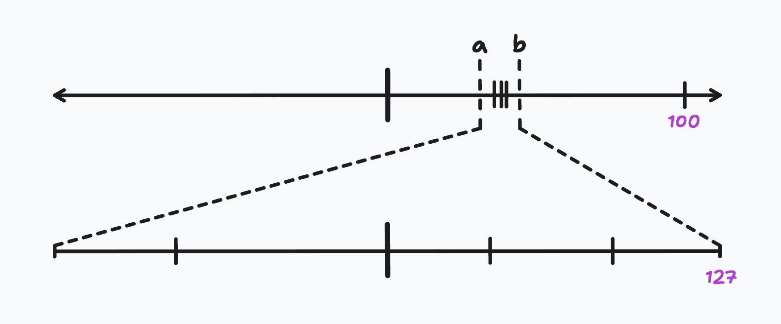
In these examples, we've defined $a$ and $b$ as the minimum and maximum float32 values in the unquantized model. This is a simple approach because it allows every float32 value to be mapped to the int8 range, but in certain cases, it may not be the best approach. For example, if the distribution of float32 values is not uniform, we may lose expressivity. Let's add a fourth float32 value to our model: 100.

In this new model, $b$ will become our new maximum float32 value, 100. Then, using the same formulas above to calculate our quantization parameters, the scaling factor $s$ becomes 0.38 and the zero point $z$ becomes -133.2. Now, when we quantize the model, here's what the quantized values look like:

Notice how skewed the new quantized values are towards both ends of the int8 range? Clearly, by including an outlier float32 value, we've sacrificed the expressivity of the quantization parameters. The best way to measure this is by dequantizing these int8 values back to float32 and then calculating their quantization errors. For example, if we quantize the float32 value 3.5 to int8 (which gives -124) and then dequantize it back to float32, we get 3.54.

This gives us a quantization error of -0.04, which is a 20x increase from the model without the outlier. The takeaway here is that we can define smarter methods to determine the quantization parameters, such as using averages or building histograms and setting $a$ and $b$ as the 1st and 99th percentiles. The range $[a, b]$ therefore becomes our clipping range, meaning that we need to clip the float32 values that fall outside of this range. With this in mind, we can redefine our mapping function as:

For example, imagine if we used a system of weighted averages to determine a clipping range $[a, b]$ that hugs the original float32 values more tightly. We'd then recalculate the quantization parameters once more with $a$ and $b$ and perform clipping on the outlier float32 value 100. This would result in a more uniform distribution of quantized values and lower quantization errors.

Quantizing in Chunks

So far, we've covered the basics of quantization by providing a simple framework to convert back and forth between float32 and quantized parameters. In our toy example above, we introduced a fictional model with only three parameters, defined the quantization parameters, and quantized the model.

However, at scale, each layer of an LLM is learning a fundamentally different role. It's therefore impractical to apply the same quantization parameters to every single parameter in the model. Such an approach would poorly fit the distribution of all float32 values in the model and we'd run into irrecoverable quantization errors.

As a result, we need a way to split up our model into smaller chunks, particularly chunks containing similarly distributed parameter values, and then derive quantization parameters for each chunk.

Per-Tensor Quantization

One of the most common ways to do this is through per-tensor quantization. A tensor in this context is synonymous with a 2D parameter matrix. Therefore, in per-tensor quantization, each parameter matrix becomes a "chunk" and receives its own quantization parameters. We derive these parameters similarly to before, but now consider every individual float32 element in the parameter matrix when choosing our clipping range.

Let's look at the definition of a linear layer (see the previous lesson for a refresher). According to the naive approach that we previously used, every parameter in the layer would be quantized using the same quantization parameters. However, with per-tensor quantization, the $W$ weights matrix and $b$ bias matrix would each have their own quantization parameters:

For other linear layers in the model, each $W$ and $b$ matrix would also receive their own quantization parameters. So, if we had a 5-layer linear model, we'd be looking at 10 sets of quantization parameters in total.

Block-Wise Quantization

In massive LLMs like Llama 2 70B, the input and output dimensions of each layer can be in the tens of thousands. This often means that we have individual weight matrices $W$ with 10M+ parameters. As we saw in the practical examples earlier, a single outlier float32 value in the matrix can significantly skew the per-tensor quantization parameters and lead to huge quantization errors.

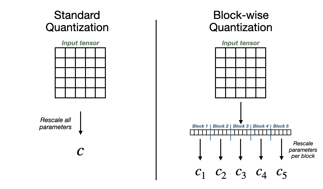
To combat this, we can employ block-wise quantization. This approach builds upon per-tensor quantization by further dividing each parameter matrix into smaller blocks.

As shown in the graphic, block-wise quantization works by flattening the parameter matrix and chopping it up into fixed-size blocks. Typically, each block will have around 32-64 matrix elements. Then, we derive quantization parameters for each block and quantize the block independently.

Llama 2 70B's attention mechanisms use weight matrices that each have ~26M parameters. With block-wise quantization, we'd calculate quantization parameters for each block of 32 weights, leading to 819,200 sets of quantization parameters for each weight matrix. While this may seem excessive, this approach is far more robust to outliers and leads to lower quantization errors across the board.