The Math Behind Quantization

Now that we know how to quantize and dequantize values, let's dive into strategies for quantizing entire LLMs. There are four common strategies: weight-only quantization, dynamic quantization, static quantization, and quantization-aware training (QAT). The first three strategies are known as post-training quantization since they quantize the model after it has been trained. Conversely, QAT is applied at training time.

Weight-Only Quantization

Weight-only quantization is a post-training quantization strategy in which the model's parameters are quantized to int8, but all operations are performed using conventional float32 matrix multiplications. It's by far the simplest of the strategies that we'll cover. Let's look once more at the formula for a single linear layer in our model that uses two float32 parameter matrices $W$ and $b$:

The first step in weight-only quantization is to derive a set of quantization parameters for each parameter matrix (remember, we're using per-tensor quantization). We start by defining the clipping ranges $[a_W, b_W]$ and $[a_b, b_b]$ for the $W$ and $b$ matrices, respectively. This can be done using one of many possible approaches, such as the naive min-max method from earlier or a more sophisticated method with averages or histograms. If we were to use the min-max method, for example, $a_W$ would be the minimum float32 value in the $W$ matrix and $b_W$ would be the maximum.

With the clipping ranges set, we then calculate the float32 scaling factors $s_W$ and $s_b$ and int8 zero points $z_W$ and $z_b$ using the standard formulas. Finally, we apply our quantization function to each parameter matrix using element-wise matrix operations:

We've now quantized the parameter matrices to int8. These steps are performed once at quantization time (also known as conversion time) in advance of inference time when we actually make predictions with the quantized model.

Now, at inference time, we only need to store the quantized parameters $W_q$ and $b_q$ in memory, reducing the layer's memory footprint by a factor of 4. When we compute the layer's output, we will dynamically dequantize the parameter matrices back to float32 using the dequantization function and then perform all the matrix operations in float32. Here's what the layer formula looks like with the quantized parameters where $D(\cdot)$ is the dequantization function:

As shown by the last equation, all we need for inference is the quantized parameter matrices and their respective quantization parameters. Then, we can generate the layer's float32 activations $Y$. While this approach is simple and greatly reduces memory, it has two drawbacks:

1. Both $X$ and $s_W (W_q - z_W)$ are float32 matrices, so their matrix multiplication is performed using float32 operations. The matrix multiplication is by far the most computationally expensive operation in the layer formula, so we're not getting the full benefit of int8 operations. Not only can GPUs move int8 data faster between their memory and chips, but they can also parallelize int8 operations more efficiently.
2. Since we're dequantizing $W_q$ and $b_q$ on the fly, we must also store the quantization parameters in memory. This is fairly negligible in our example using per-tensor quantization since even the largest LLMs only have around ~100 layers, but it will become an important consideration in later discussions.

Dynamic Quantization

Dynamic quantization is an upgraded version of weight-only quantization where we also quantize the layer's activations at inference time. This is done entirely on the fly (hence, "dynamic") and gives us the benefit of performing most matrix operations in int8.

What does it mean to quantize our activations? Let's think about the float32 activations matrix $Y$ that is outputted by our layer formula. Similar to how we derived the quantization parameters for the parameter matrices $W$ and $b$ at conversion time, we can choose a clipping range $[a_Y, b_Y]$ and derive the quantization parameters $s_Y$ and $z_Y$ at inference time. Then, we can dynamically quantize $Y$ to int8:

Finally, all we have to do is pass the quantized activations and their quantization parameters to the next layer: $X_q = Y_q$, $s_X = s_Y$, and $z_X = z_Y$. Now, we can completely rewrite the layer formula by also dynamically dequantizing our new $X_q$ in addition to $W_q$ and $b_q$:

This new layer definition might look way more complex, but we've done something super cool here. By reframing the layer formula this way, we can perform the layer's matrix multiplication between $X_q$ and $W_q$ entirely using int8 operations. In fact, all operations between the square brackets can be done in int8 since the zero point parameters are also int8! We therefore reap the same benefits of reduced memory as weight-only quantization, but also cut down the inference latency due to the optimized integer ops.

In the layer formula, we scale the int8 calculations back to float32 with the scaling factors $s_X$, $s_W$, and $s_b$ and apply the $\text{tanh}(\cdot)$ activation function to generate the float32 activations $Y$. We can then rinse and repeat by once again dynamically quantizing $Y$ into $Y_q$ and feeding it to the subsequent layer in the model.

Static Quantization

Static quantization builds off dynamic quantization by determining the quantization parameters for the activations at conversion time instead of inference time. Basically, instead of defining the clipping range $[a_Y, b_Y]$ on the fly using the layer's exact float32 activations $Y$, we effectively "guess" the clipping range by simulating the model on representative data. We call this process calibration.

Calibration works by taking a small subset of unlabeled samples from the training or validation sets (usually between 100-500) and running them through the unquantized float32 model. We can then observe the range of float32 values that each activations matrix $Y$ experiences and set the clipping range $[a_Y, b_Y]$ accordingly using one of the methods we discussed (e.g. min-max, moving averages, histograms, etc). Finally, we calculate the scaling factor $s_Y$ and zero point $z_Y$ for each activations matrix $Y$ in the model before any activations are actually computed at inference time.

Since we know $s_Y$ and $z_Y$ ahead of time, we can update our layer formula to directly output the quantized activations $Y_q$. This is a big improvement over dynamic quantization which outputs a float32 activations matrix $Y$ that is only then quantized to $Y_q$.

What is so cool about this new layer formula? It can be computed entirely in int8! Also, we no longer need to dynamically quantize the activations during inference, which saves us even more time. Finally, we completely avoid storing the float32 activations $Y$ in memory when moving between layers, which further reduces the model's memory footprint.

Before moving on, one caveat to note is that static quantization will never be as accurate as dynamic quantization (i.e. it will result in higher quantization errors). This is because the clipping ranges $[a_Y, b_Y]$ are smart guesses based on the calibration data, but they will never be as perfect as using the exact float32 activations at inference time like in dynamic quantization. We're therefore sacrificing a bit of accuracy for speed and memory savings.

Quantization-Aware Training

When we quantize and subsequently dequantize a float32 value, we experience a loss of information. Earlier, we expressed this as the following quantization error:

Quantization-aware training (QAT) offers an alternative to post-training quantization techniques by adapting the model to the quantization process during training. QAT effectively teaches the model to take the quantization error into account when updating its parameters, which leads to a more accurate quantized model at inference time.

To make this work, we add two new layers around each existing layer of a normal pre-trained model: a quantization layer (Q) and a dequantization layer (DQ). These new layers will simulate the quantization error that a post-training quantized model typically experiences at inference time.

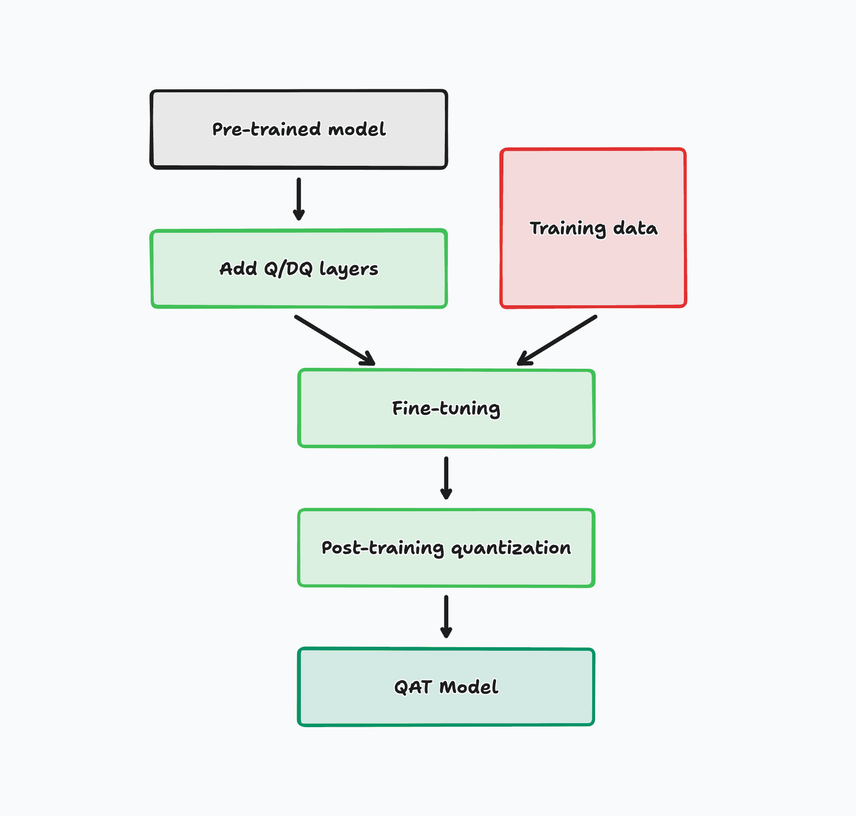
We then fine-tune the model on new training data and let the model adapt its parameters to the simulated quantization error. Note that this process is performed entirely in float32 and the quantization layers are merely simulating the effects of quantization. We're not actually quantizing the model during training.

Finally, we quantize the model using one of the three post-training quantization techniques that we learned about. The model will now be far more robust to any quantization error that it experiences at inference time and should perform better than any post-training quantization technique.

Summary

To summarize, below is a table with the four quantization strategies that we've learned about and their relative strengths and weaknesses. In the next section, we'll learn how these separate strategies are implemented by open-source quantization libraries and how to implement them in practice.